qnorm(0.025, mean = 0, sd = 1) # N(0, 1)[1] -1.959964qgamma(0.025, shape = 10, rate = 10) # Gamma(10, 10)[1] 0.4795389
Q: How can we quantify the uncertainty in our estimates?
A: Think back to STAT 155…
Goal: Quantify how much our estimates vary from sample to sample.
We’ve already seen how to derive these! \[\text{SE}(\hat\theta) = \sqrt{\text{Var}(\hat\theta)}\]
Goal: Provide a range of plausible values for the unknown parameter.
(Bonus: the width of the interval also communicates amount of uncertainty in our estimate.)
Questions we’ll answer in this class:
FYI: We will see some nice connections to our recent discussions about asymptotic properties!
Suppose \(Y_1, \dots, Y_n\) are a random sample from a distribution with unknown mean \(\mu\) and known variance \(\sigma^2\). Derive a 95% CI for \(\mu\).
Thanks to the CLT, we know \[\sqrt{n}\left(\bar{Y} - \mu\right) \stackrel{d}{\to} N(0, \sigma^2),\] or equivalently, \[\sqrt{n}\left(\frac{\bar{Y} - \mu}{\sigma}\right) \stackrel{d}{\to} N(0, 1).\]
Thus, for large enough \(n\), we can say that \[\sqrt{n}\left(\frac{\bar{Y} - \mu}{\sigma}\right) \dot\sim N(0, 1),\] ie \(\sqrt{n}\left(\frac{\bar{Y} - \mu}{\sigma}\right)\) is “approximately” normally distributed.
This means that \[0.95 \approx \Pr\left(-1.96 < \sqrt{n}\left(\frac{\bar{Y} - \mu}{\sigma}\right) < 1.96 \right).\] (Recall the 68-95-99.7 rule for normal distributions!)
Rearranging this statement we get, \[ \begin{align*} 0.95 &\approx \Pr\left(-1.96 \le \sqrt{n}\left(\frac{\bar{Y} - \mu}{\sigma}\right) \le 1.96 \right) \\ & = \Pr\left(-1.96 \frac{\sigma}{\sqrt{n}} \le \bar{Y} - \mu \le 1.96 \frac{\sigma}{\sqrt{n}} \right) \\ & = \Pr\left( - \bar{Y} -1.96 \frac{\sigma}{\sqrt{n}} \le -\mu \le - \bar{Y} + 1.96 \frac{\sigma}{\sqrt{n}} \right) \\ & = \Pr\left(-\left[ - \bar{Y} -1.96 \frac{\sigma}{\sqrt{n}}\right] \ge \mu \ge -\left[- \bar{Y} + 1.96 \frac{\sigma}{\sqrt{n}} \right] \right) \\ & = \Pr\left(\bar{Y} + 1.96 \frac{\sigma}{\sqrt{n}} \ge \mu \ge \bar{Y} - 1.96 \frac{\sigma}{\sqrt{n}}\right). \\ \end{align*} \]
Thus, \(\left(\bar{Y} - 1.96 \frac{\sigma}{\sqrt{n}}, \bar{Y} + 1.96 \frac{\sigma}{\sqrt{n}}\right)\) is an (approximate) 95% CI for \(\mu\).
Notice that this CI takes the familiar form from STAT 155, \(\text{estimate} \pm 2 \times \text{SE}\):
At your tables, discuss:
Suppose \(Y_1, \dots, Y_n \stackrel{iid}{\sim} \text{Exponential}(\lambda)\), where \[f_Y(y\mid \lambda) = \lambda e^{-\lambda y}, y > 0, \lambda > 0.\] Construct a 95% confidence interval for \(\lambda\) using an exact pivot. We’ll break this into a few steps…
Is \(Z = \sum_{i=1}^n Y_i\) an exact pivotal quantity for \(\lambda\)? Why or why not?
HINT: \(Y_i \stackrel{iid}{\sim} \text{Exponential}(\lambda)\) \(\implies\) \(\sum_{i=1}^n Y_i \sim \text{Gamma}(n,\lambda)\)
How about \(W = \frac{\lambda}{n}\sum_{i=1}^n Y_i\)? Why/why not?
HINT: \(Y_i \stackrel{iid}{\sim} \text{Exponential}(\lambda)\) \(\implies\) \(\frac{\lambda}{n}\sum_{i=1}^n Y_i \sim \text{Gamma}(n,n)\)
Make a probability statement involving the pivotal quantity and use it to derive a \(100(1-\alpha)\)% confidence interval for \(\lambda\). Use the notation \(q_a\) to represent the \(a\)th quantile of the involved distribution.
Consider the example problem above. What happens if we don’t know \(\sigma^2\)? Do we run into any issues here? If yes, what should we do?
HINT: Use your work from PS4 Question 4 to help you here!
Propose a pivotal quantity (and confirm it is, in fact, a pivot).
To do this, you’ll either need to find the exact distribution of your pivot, using techniques from MATH/STAT 354: Probability, or you can find the approximate distribution of your pivot using tools from this class (CLT, Delta Method, Slutsky’s Theorem).
Write down a probability statement involving the quantiles of your pivot’s (exact or approximate) distribution: \(1- \alpha = \Pr(q_{\alpha/2} \le g(\mathbf{Y},\theta) \le q_{1-\alpha/2})\).
If the distribution is Normal, use the 68-95-99.7 rule! Otherwise, you need to figure out the quantiles of your distribution, using techniques from MATH/STAT 354 and/or R (qbinom, qgamma, etc.).
Re-arrange until you have a probability statement involving the unknown parameter on its own: \(1 - \alpha = \Pr(??? \le \theta \le ???)\).
Propose a pivotal quantity and confirm that it is in fact a pivot: function of data and unknown parameter, distribution doesn’t depend on unknown parameter
EXAMPLE 1: \(\sqrt{n}\left( \frac{\bar{X} - \mu}{S}\right) \overset{d}{\to} N(0,1)\)
EXAMPLE 2: \(\frac{\lambda}{n} \sum_{i=1}^n Y_i \sim \text{Gamma}(n,n)\)
Write down a probability statement involving the quantiles of our pivot’s distribution, \[1-\alpha = \Pr(q_{\alpha/2} \le g(\mathbf{Y}, \theta) \le q_{1 - \alpha/2})\]
EXAMPLE 1: \(0.95 = \Pr(-1.96 \le Z \le 1.96)\) if \(Z \sim N(0,1)\)
EXAMPLE 2: \(0.95 = \Pr(q_{0.025} \le W \le q_{0.975})\), where \[a = \int_{0}^{q_a} \frac{n^n}{\Gamma(n)}w^{n-1}e^{-nw} dw\]
Can use R to help find quantiles!
qnorm(0.025, mean = 0, sd = 1) # N(0, 1)[1] -1.959964qgamma(0.025, shape = 10, rate = 10) # Gamma(10, 10)[1] 0.4795389
Many of the confidence intervals we construct using pivots rely on asymptotic results: \(\overset{d}{\to}\) rather than \(\sim\).
EXAMPLE:
If \(n\) is large, these “approximate” CIs work well!
But if \(n\) is too small, our asymptotic results won’t have “kicked in” yet, and the CI could be wrong.
In those cases, it’s desirable to have an exact CI that doesn’t rely on asymptotic results. This will require knowing exact, finite sample distributions.
EXAMPLES:
Let \(X_1, \dots, X_n\) be a random sample from a Bernoulli distribution with probability of success \(p\).
Construct a 95% CI for \(p\) using \(Z_1 = \frac{\hat{p}-p}{\sqrt{p(1-p)/n}}\) as an approximate pivot, where \(\hat{p} = \frac{1}{n} \sum_{i=1}^n X_i\).
Confirm \(Z_1\) is in fact an approximate pivot. (HINT: CLT)
Try to construct a 95% CI for \(p\) using this pivot. Do you run into any issues?
Next, construct a 95% CI for \(p\) using \(Z_2 = \frac{\hat{p}-p}{\sqrt{\hat{p}(1-\hat{p})/n}}\) as an approximate pivot.
Confirm this is an approximate pivot. (HINT: CLT + WLLN + CMT + Slutsky’s)
Use this pivot to construct a 95% CI for \(p\).
\(Z_1 = \frac{\hat{p}-p}{\sqrt{p(1-p)/n}}\)
Yes, \(Z_1\) is an approximate pivot. It depends on the data (\(\hat{p} = \bar{X}\)) and the unknown parameter, \(p\). By the CLT, we know \(Z_1 \overset{d}{\to} N(0,1)\). Thus, the (asymptotic) distribution of \(Z_1\) does not depend on \(p\).
We start by writing down a probability statement involving \(Z_1\): \[ \begin{align*} 0.95 &\approx \Pr(-1.96 \le \frac{\hat{p}-p}{\sqrt{p(1-p)/n}} \le 1.96) \\ & = \dots \\ & = \Pr\left(\hat{p} - 1.96 \sqrt{p(1-p)/n} \le p \le \hat{p} + 1.96 \sqrt{p(1-p)/n}\right) \end{align*} \] But this doesn’t work as a CI! The lower and upper bounds of this interval still involve \(p\), which we don’t know. Can you find a way to re-arrange further to isolate \(p\)? (I couldn’t!)
\(Z_2 = \frac{\hat{p}-p}{\sqrt{\hat{p}(1-\hat{p})/n}}\)
First, note that \[ \frac{\hat{p}-p}{\sqrt{\hat{p}(1-\hat{p})/n}} = \left(\frac{\hat{p}-p}{\sqrt{p(1-p)/n}}\right) \left(\frac{\sqrt{p(1-p)}}{\sqrt{\hat{p}(1-\hat{p})}}\right) \] We know that the first term converges in distribution to \(N(0,1)\) thanks to the CLT. For the second term, consider the denominator. The WLLN tells us \(\hat{p} = \bar{X} \overset{p}{\to} E(X) = p\). By the continuous mapping theorem, it follows that \(\sqrt{\hat{p}(1-\hat{p})} \overset{p}{\to} \sqrt{p(1-p)}\). Combining this with Slutsky’s Theorem, we know that the second term is converging in probability to \(1\). Thus, using Slutsky’s Theorem again, we know \[ \frac{\hat{p}-p}{\sqrt{\hat{p}(1-\hat{p})/n}} \overset{d}{\to} \left[ N(0, 1) \right] \left[ 1 \right] \overset{d}{=} N(0, 1) \] So, yes, \(Z_2\) is an approximate pivot! It depends on the data and \(p\), and its approximate distribution does not depend on \(p\).
Our 95% CI for \(p\) is: \[ \begin{align*} 0.95 &\approx \Pr\left(-1.96 \le \frac{\hat{p}-p}{\sqrt{\hat{p}(1-\hat{p})/n}} \le 1.96 \right) \\ & = \dots \\ & = \Pr\left(\hat{p} - 1.96 \sqrt{\frac{\hat{p}(1-\hat{p})}{n}} \le p \le \hat{p} + 1.96 \sqrt{\frac{\hat{p}(1-\hat{p})}{n}} \right) \end{align*} \]
To find an interval estimate for \(p\) without resorting to a CLT-based Normal approximation, we can use what we know about the exact distribution of \(X = \sum_{i=1}^n X_i\) instead. What’s the distribution of \(X\)?
Is \(X\) an exact pivot? If not, do you have any ideas on how you could modify \(X\) to create an exact pivot?
Stuck on the second part of the last question? Me too! Let’s try something else…
Download this QMD file and complete the rest of the activity in R.
\(X \sim \text{Binomial}(n, p)\)
\(X\) is not an exact (or approximate) pivot. It’s not a function of \(p\), and its distribution does depend on \(p\). I couldn’t come up with any ideas on how to modify \(X\) to get a pivot — could you?
See here: Activity Solutions (but don’t peek at Part 2!)
After class today…
Continue wherever you left off last Friday.
Goal for today: compare the exact and approximate CIs using a simulation study!
Coverage simulations are a useful way to assess if a proposed confidence interval construction process is working.
If we have a method that is supposed to yield a 95% confidence interval, then when we repeat this method across repeated samples we should see that the resulting CIs actually cover the true parameter 95% of the time. If not, that’s a problem!
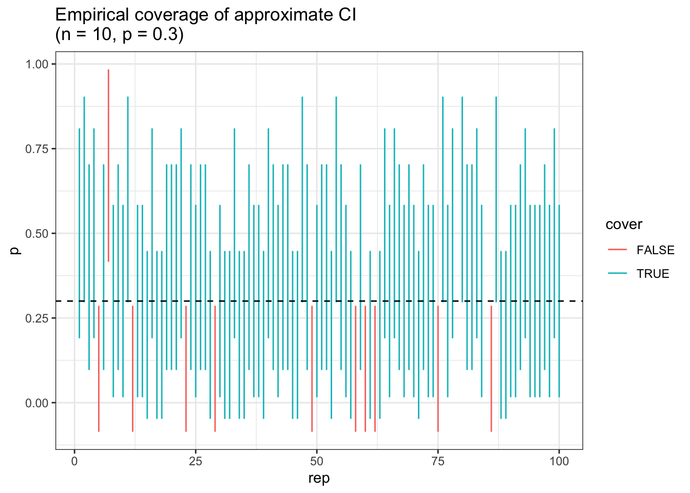
Coverage = how often (across repeated samples from the population) does the confidence interval actually contain the true parameter?
When we talk about a 95% probability, we’re talking about the performance (ie coverage) of this interval construction process across repeated samples. \[\Pr\left(\hat{p}-1.96\sqrt{\frac{\hat{p}\left(1-\hat{p}\right)}{n}} \le p \le \hat{p}+1.96\sqrt{\frac{\hat{p}\left(1-\hat{p}\right)}{n}}\right) \approx 0.95\] \[\hat{p} = \frac{1}{n}\sum_{i=1}^n X_i\]
For the interval resulting from a single sample, \(p\) is either in the observed interval or not. There’s nothing random! \[\Pr\left(p_e-1.96\sqrt{\frac{p_e\left(1-p_e\right)}{n}} \le p \le p_e+1.96\sqrt{\frac{p_e\left(1-p_e\right)}{n}}\right) \in \{0, 1\}\] \[p_e = \frac{1}{n}\sum_{i=1}^n x_i\]