11 Consistency
An Asymptotic Property
Day 1
Settling In
- Sit anywhere you want!
- Catch up on Slack
Where Are We?
So far this semester, we’ve talked about (1) constructing estimators and (2) assessing the behavior of those estimators.
Our discussion of (2) has thus far focused on finite sample properties, eg:
- bias / unbiasedness
- variance / efficiency
- sufficiency
But it’s also interesting to explore what happens as we collect more and more data (\(n \rightarrow \infty\)), eg:
- asymptotic unbiasedness (PS2 Problem 7)
- consistency (today)
- asymptotic efficiency (coming soon!)
- asymptotic normality (coming soon!)
There are known as asymptotic properties.
Consistency
- Consistent
- \(\hat\theta_n\) is a consistent estimator for \(\theta\) if, for any \(\epsilon > 0\), \[\lim_{n \rightarrow \infty} \Pr( \lvert \hat\theta_n - \theta \rvert < \epsilon) = 1,\] or, equivalently, \[\lim_{n \rightarrow \infty} \Pr( \lvert \hat\theta_n - \theta \rvert \ge \epsilon) = 0.\]
(Note the use of a subscript \(n\) to remind ourselves that our estimator depends on the sample size!)
- Consistent (\(\epsilon, \delta\) version)
- \(\hat\theta_n\) is a consistent estimator for \(\theta\) if, for any \(\epsilon > 0\) and \(\delta > 0\), there exists \(n(\epsilon, \delta)\) such that \[\Pr(\lvert \hat\theta_n - \theta \rvert < \epsilon) > 1 - \delta \text{ for } n > n(\epsilon, \delta)\]
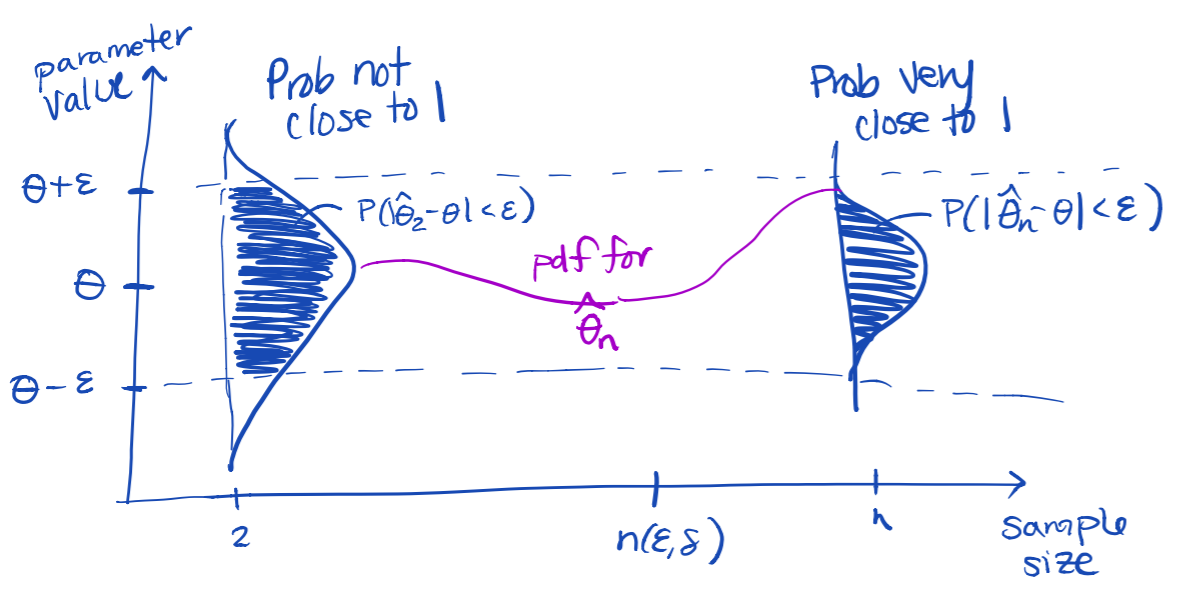
Intuition 💡
Consistency tells us that our estimator will “always” (with probability approach 1) be close to the truth as the sample size increases
Proving Estimators are Consistent
Use the definition (limit version or \(\epsilon, \delta\) version)
Since MATH 377: Real Analysis is not a prerequisite for this course, we won’t do many examples like this. (See Consistency Examples video for one!) But, if you have taken Real Analysis, practicing proving that estimators are consistent using this approach would be a worthwhile endeavor outside of class time!
Show that an estimator is either unbiased or asymptotically unbiased, and that the variance is going to zero. Thanks to Chebyshev’s Inequality (and its corollaries), this is “sufficient” (pun intended) for proving an estimator is consistent.
Chebyshev’s Inequality and Corollaries
- Chebyshev’s Inequality
- Let \(W\) be a random variable with mean \(\mu\) and variance \(\sigma^2\). For any \(\epsilon > 0\), \[\Pr(\lvert W - \mu \rvert < \epsilon) \ge 1 - \frac{\sigma^2}{\epsilon^2},\] or, equivalently, \[\Pr(\lvert W - \mu \rvert \ge \epsilon) \le \frac{\sigma^2}{\epsilon^2}.\]
Intuition 💡
Chebyshev’s Inequality gives us a lower bound on the probability that a random variable is close to its mean or, likewise, an upper bound on the probability that the random variable is far from its mean.
Proof
See today’s board notes.
- Corollary 1
- If \(\hat\theta_n\) is an unbiased estimator for \(\theta\) and \(\lim_{n\rightarrow\infty} \text{Var}(\hat\theta_n) = 0\), then \(\hat\theta_n\) is consistent for \(\theta\).
Proof
See today’s board notes.
- Corollary 2
- If \(\hat\theta_n\) is an asymptotically unbiased estimator for \(\theta\) and \(\lim_{n\rightarrow\infty} \text{Var}(\hat\theta_n) = 0\), then \(\hat\theta_n\) is consistent for \(\theta\).
Proof
on your next problem set :)
Wrapping Up
General Tips for Writing Proofs
Start by writing what you know (eg assume your assumptions are true).
(If the theorem involves something being true for all values of \(\epsilon\) greater than 0, letting \(\epsilon\) be greater than 0 will be your next step.)
Then, write what you’re trying try to show, using mathematical notation.
Use related definitions, theorems, and properties wherever you can.
Examples:
- \(\text{Var}(Y) = E(Y^2) - E^2(Y)\)
- \(E(Y) = \int y f(y) dy\)
- \(f(y) \ge 0\) and \(\int f(y) dy = 1\)
- sandwich/squeeze theorem
It should always be clear how you’re getting from one line to the next, including when you are using your assumptions. Use text to supplement/clarify!
After Class Today…
FYI: Your next problem set, PS4, will be due March 30. I’ll post it when we get back from break.
Day 2
Welcome back from Spring Break! ☀️
Settling In
- Catch up on recent Slack messages
- Note the slightly revised schedule:
- no checkpoint this week
- PS4 deadline: March 30 -> April 1
- Quiz 4: April 6 -> April 8
- Review your notes on consistency and prepare to discuss!
Checkpoint Discussion
At your table, discuss:
What’s the difference between a finite sample versus asymptotic property of an estimator? Provide an example of each.
Intuitively, what does it mean for an estimator to be consistent?
Write down the definition of consistency using mathematical notation.
Describe the connections between the following properties (eg which implies the other?):
- unbiased
- asymptotically unbiased
- consistent
How can we use Chebyshev’s Inequality to show that an estimator is consistent?
Solutions
Finite sample properties (eg bias, variance, MSE, efficiency, sufficiency) look at how an estimator behaves for a fixed, finite sample size \(n < \infty\). Asymptotic properties (eg asymptotic bias, consistency) consider what happens to the estimator as the sample size gets very large \(n \rightarrow \infty\).
When our sample size gets large enough, our estimates will be almost always (with probability approaching 1) close to the truth.
\(\hat\theta_n\) is a consistent estimator of \(\theta\) if \[\lim_{n\rightarrow\infty} \Pr(\lvert \hat\theta_n - \theta \rvert < \epsilon) = 1 \quad \forall \epsilon > 0,\] or, equivalently, \[\lim_{n\rightarrow\infty} \Pr(\lvert \hat\theta_n - \theta \rvert \ge \epsilon) = 0 \quad \forall \epsilon > 0.\]
connections:
- unbiased \(\implies\) asymptotically unbiased (but the reverse is not true)
- unbiased plus var \(\rightarrow 0\) \(\implies\) consistent (but unbiased, alone, does not imply consistent)
- asymptotically unbiased plus var \(\rightarrow 0\) \(\implies\) consistent (but asymptotically unbiased, alone, does not imply consistent)
- consistent \(\nRightarrow\) unbiased (you can construct an estimator that is consistent but not unbiased, eg Practice Problems #1)
- consistent \(\nRightarrow\) asymptotically unbiased (you can construct an estimator that is consistent but not asymp unbiased, eg \(\hat\theta_n = 0\) with probability \(\frac{n-1}{n}\) and \(n\) with prob. \(\frac{1}{n}\) where we are trying to estimate \(\theta = 0\))
Show the variance of the estimator approaches zero as \(n \rightarrow \infty\) and the estimator is either unbiased (Corollary 1) or asymptotically unbiased (Corollary 2).
Practice Problems
Suppose \(Y_1, \dots, Y_n\) are a random sample from a distribution with mean \(\mu\) and variance \(\sigma^2\). Which of the following estimators are consistent for \(\mu\)?
- \(\hat\mu_1 = \overline{Y}\)
- \(\hat\mu_2 = \overline{Y} + \frac{1}{n}\)
- \(\hat\mu_3 = Y_1\)
- \(\hat\mu_4 = Y_1 + \frac{1}{n}\)
NOTE: If an estimator does not satisfy the conditions necessary to use one of the Chebyshev’s Inequality Corollaries, think about how you would show it is not consistent, but no need to actually formally prove it is not.
Suppose \(Y_1, \dots, Y_n \stackrel{iid}{\sim} \text{Unif}(0, \theta)\). In the Consistency Examples Video, we showed that the MLE, \(\hat\theta_{MLE} = Y_{(n)}\), is a consistent estimator of \(\theta\) using the definition of consistency and techniques from calculus. Now, use a corollary of Chebyshev’s Inequality to show that \(\hat\theta_{MLE}\) is consistent.
HINT: Recall that \(f_{Y_{(n)}}(y) = n \theta^{-n} y^{n-1}, 0 \le y \le \theta\).
Solutions
See today’s board notes.
Wrapping Up
Consistency Debrief
Consistency is a nice property for an estimator to have! It tells us that, as our sample size gets larger, we have a very high probability of “getting it right” (or at least close to it)
Chebyshev’s Inequality makes it a lot easier to prove consistency.
The Practice Problems show us that a consistent estimator is not necessarily (asymptotically) unbiased, and an (asymptotically) unbiased estimator is not necessarily consistent!
There are other asymptotic properties that we like to see in estimators. More on this in the class periods to come!