4 Linear Regression
Connecting Least Squares and Maximum Likelihood Estimation
Settling In
- Check out the actually finalized OH schedules: Kelsey | Nick
- If my office hours don’t work for you, please post questions on Slack and/or set up a one-on-one appointment!
- Check Slack for recent messages
- Get started on the Checkpoint Discussion questions, below
Checkpoint Discussion
CP2 covers the following content:
- Linear Algebra Review!
- (specially: matrix multiplication, transposes, inverses, and determinants)
Consider the following vectors and matrices:
\[ \mathbf{y} = \begin{bmatrix} y_1 \\ y_2 \\ \vdots \\ y_n \end{bmatrix}, \quad \boldsymbol\epsilon = \begin{bmatrix} \epsilon_1 \\ \epsilon_2 \\ \vdots \\ \epsilon_n \end{bmatrix}, \quad \boldsymbol\beta = \begin{bmatrix} \beta_0 \\ \beta_1 \\ \vdots \\ \beta_p \end{bmatrix}, \quad \mathbf{X} = \begin{bmatrix} 1 & x_{11} & x_{21} & \dots & x_{p1} \\ 1 & x_{12} & x_{22} & \dots & x_{p2} \\ \vdots & \vdots & \vdots & \ddots & \vdots \\ 1 & x_{1n} & x_{2n} & \dots & x_{pn} \end{bmatrix} \]
Work on the following questions with your table:
What are the dimensions of the product \(\mathbf{X} \boldsymbol\beta\)?
Find the top left entry of the product \((\mathbf{X} \boldsymbol\beta)_{11}\)
“FOIL” / expand the following: \((\mathbf{y} - \mathbf{X}\boldsymbol\beta)^\top (\mathbf{y} - \mathbf{X}\boldsymbol\beta)\)
What questions do you still have about CP2?
Solutions
\(\mathbf{X}\) is \(n \times (p+1)\) and \(\boldsymbol\beta\) is \((p+1) \times 1\), so \(\mathbf{X}\boldsymbol\beta\) will be \(n \times 1\)
The top left entry is highlighted in red below:
\[ \begin{align*} \mathbf{X}\boldsymbol\beta & = \begin{bmatrix} 1 & x_{11} & x_{21} & \dots & x_{p1} \\ 1 & x_{12} & x_{22} & \dots & x_{p2} \\ \vdots & \vdots & \vdots & \ddots & \vdots \\ 1 & x_{1n} & x_{2n} & \dots & x_{pn} \end{bmatrix} \begin{bmatrix} \beta_0 \\ \beta_1 \\ \beta_2 \\ \vdots \\ \beta_p \end{bmatrix} \\ & = \begin{bmatrix} \color{red}{\beta_0 + \beta_1 x_{11} + \beta_2 x_{21} + \dots \beta_p x_{p1}} \\ \beta_0 + \beta_1 x_{12} + \beta_2 x_{22} + \dots \beta_p x_{p2} \\ \vdots \\ \beta_0 + \beta_1 x_{1n} + \beta_2 x_{2n} + \dots \beta_p x_{pn} \end{bmatrix} \\ \end{align*} \]
- We can expand this out as follows:
\[ \begin{align*} (\mathbf{y} - \mathbf{X}\boldsymbol\beta)^\top (\mathbf{y} - \mathbf{X}\boldsymbol\beta) & = ((\mathbf{y})^\top - (\mathbf{X}\boldsymbol\beta)^\top) (\mathbf{y} - \mathbf{X}\boldsymbol\beta) \\ & = (\mathbf{y}^\top - \boldsymbol\beta^\top \mathbf{X}^\top) (\mathbf{y} - \mathbf{X}\boldsymbol\beta) \\ & = \mathbf{y}^\top \mathbf{y} - \mathbf{y}^\top \mathbf{X}\boldsymbol\beta - \boldsymbol\beta^\top \mathbf{X}^\top \mathbf{y} + \boldsymbol\beta^\top \mathbf{X}^\top \mathbf{X}\boldsymbol\beta \\ & = \mathbf{y}^\top \mathbf{y} - 2\mathbf{y}^\top \mathbf{X}\boldsymbol\beta + \boldsymbol\beta^\top \mathbf{X}^\top \mathbf{X}\boldsymbol\beta, \\ & \quad \quad \text{ because } \mathbf{y} \text{ and } \mathbf{X}\boldsymbol\beta \text{ are } (n \times 1) \text{ vectors } \end{align*} \]
We’ll multiply this out later!
Useful Matrix Properties
Multiplication:
- \((\mathbf{A} + \mathbf{B})\mathbf{C} = \mathbf{A}\mathbf{C} + \mathbf{B}\mathbf{C}\)
- \(\mathbf{A}\mathbf{B} \neq \mathbf{B}\mathbf{A}\) (order matters!)
Transposes:
- \((\mathbf{A} + \mathbf{B})^\top = \mathbf{A}^\top + \mathbf{B}^\top\)
- \((\mathbf{A}\mathbf{B})^\top = \mathbf{B}^\top \mathbf{A}^\top\)
- \(\mathbf{a}^\top \mathbf{b} = \mathbf{b}^\top \mathbf{a}\)
Inverses:
- \(\mathbf{A}\mathbf{A}^{-1} = \mathbf{A}^{-1}\mathbf{A} = \mathbf{I}\)
- \(\mathbf{I}^{-1} = \mathbf{I}\)
- \(\mathbf{A} \mathbf{B} = \mathbf{C} \implies \mathbf{B} = \mathbf{A}^{-1} \mathbf{C}\) \(\quad\) (if \(\mathbf{A}^{-1}\) exists)
- \((\mathbf{A}\mathbf{B})^{-1} = \mathbf{B}^{-1} \mathbf{A}^{-1}\)
Determinants:
- \(\det(\mathbf{A}) = ad - bc\) for a \(2 \times 2\) matrix \(\mathbf{A} = \begin{bmatrix} a & b \\ c & d \end{bmatrix}\)
- \(\det(\mathbf{I}_{n\times n}) = 1\)
- \(\det\left(c\mathbf{I}_{n\times n}\right) = c^n\)
Check out the Matrix Cookbook resource linked on Moodle for more!
Linear Regression with Matrices
Least Squares Estimation
Simple Linear Regression (Day 1 Review)
Suppose we have the simple linear regression model \[y_i = \beta_0 + \beta_1 x_i + \epsilon_i, \ i = 1, ..., n\]
To find the least squares estimates for the unknown intercept (\(\beta_0\)) and slope (\(\beta_1\)), we minimize the sum of squared errors (SSE):
\[ (\hat\beta_0, \hat\beta_1) = \arg\min_{\beta_0, \beta_1} \text{SSE} = \arg\min_{\beta_0, \beta_1} \sum_{i=1}^n \left(y_i - [\beta_0 + \beta_1 x_i] \right)^2 \]
Example:
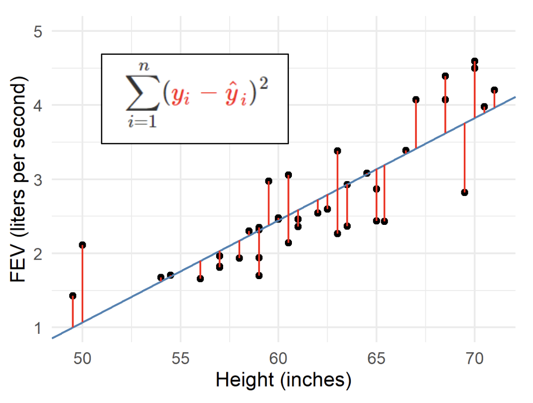
Finding these estimates involves the following steps:
- Find the partial derivatives with respect to each unknown parameter \(\frac{\partial}{\partial \beta_0} \text{SSE}, \frac{\partial}{\partial \beta_1} \text{SSE}\)
- Set those partial derivatives equal to zero and solve for \(\beta_0, \beta_1\).
Result:
\[ \begin{align*} \hat\beta_0 &= \bar{y} - \hat\beta_1 \bar{x} \\ & \\ & \text{and} \\ & \\ \hat\beta_1 & = \frac{\sum_{i=1}^n y_i x_i - n\bar{y}\bar{x}}{\sum_{i=1}^n x_i^2 - n\bar{x}^2}\\ & = \frac{\sum_{i=1}^n (y_i - \bar{y})(x_i - \bar{x})}{\sum_{i=1}^n (x_i - \bar{x})^2} \\ \end{align*} \]
Why are the last two lines equivalent?
Let’s focus on the numerator to start: \[ \begin{align*} \sum_{i=1}^n (y_i - \bar{y})(x_i - \bar{x}) & = \sum_{i=1}^n (y_i x_i - \bar{y} x_i - \bar{x} y_i + \bar{x}\bar{y}) \\ & = \sum_{i=1}^n (y_i x_i) - \sum_{i=1}^n(\bar{y} x_i) - \sum_{i=1}^n(\bar{x} y_i) + \sum_{i=1}^n(\bar{x}\bar{y}) \\ & = \sum_{i=1}^n y_i x_i - \bar{y}\sum_{i=1}^n x_i - \bar{x}\sum_{i=1}^n y_i + n\bar{x}\bar{y} \\ & = \sum_{i=1}^n y_i x_i - \bar{y} \left(n \frac{1}{n}\right) \sum_{i=1}^n x_i - \bar{x} \left(n \frac{1}{n}\right) \sum_{i=1}^n y_i + n\bar{x}\bar{y} \\ & = \sum_{i=1}^n y_i x_i - \bar{y} n \left(\frac{1}{n} \sum_{i=1}^n x_i \right) - \bar{x} n \left(\frac{1}{n} \sum_{i=1}^n y_i \right) + n\bar{x}\bar{y} \\ & = \sum_{i=1}^n y_i x_i - \bar{y} n \left( \bar{x} \right) - \bar{x} n \left( \bar{y}\right) + n\bar{x}\bar{y} \\ & = \sum_{i=1}^n y_i x_i - n \bar{x}\bar{y} - n \bar{x}\bar{y} + n\bar{x}\bar{y} \\ & = \sum_{i=1}^n y_i x_i - n\bar{y}\bar{x} \end{align*} \] Follow similar steps for the denominator!
Multiple Linear Regression
Now, imagine we have \(p\) predictors: \[y_i = \beta_0 + \beta_1 x_{1i} + \beta_2 x_{2i} + \dots + \beta_p x_{pi} + \epsilon_i, \quad i = 1, ..., n\]
Our least squares estimation problem becomes: \[(\hat\beta_0, ..., \hat\beta_p) = \arg \min_{\beta_0, ... \beta_p} \sum_{i=1}^n \left( y_i - \left[\beta_0 + \beta_1 x_{1i} + \dots + \beta_p x_{pi} \right]\right)^2\]
This gets complicated quickly! Enter: matrices.
Multiple Linear Regression with Matrices
We can re-write our linear regression model using vectors and matrices: \[\mathbf{y} = \mathbf{X}\boldsymbol\beta + \boldsymbol\epsilon,\] with \(\mathbf{y}, \mathbf{X}, \boldsymbol\beta, \boldsymbol\epsilon\) as defined above.
With this notation, the least squares estimation problem becomes: \[\hat{\boldsymbol\beta} = \arg\min_{\boldsymbol\beta} \text{SSE} = \arg\min_{\boldsymbol\beta} (\mathbf{y} - \mathbf{X}\boldsymbol\beta)^\top (\mathbf{y} - \mathbf{X}\boldsymbol\beta)\]
We solve this problem by finding the derivative of \((\mathbf{y} - \mathbf{X}\boldsymbol\beta)^\top (\mathbf{y} - \mathbf{X}\boldsymbol\beta)\) with respect to the vector \(\boldsymbol\beta\), setting that derivative equal to a vector of zeroes, and solving: \[
\begin{align*}
\frac{\partial}{\partial{\boldsymbol\beta}} (\mathbf{y} - \mathbf{X}\boldsymbol\beta)^\top (\mathbf{y} - \mathbf{X}\boldsymbol\beta) \equiv \mathbf{0} \\
\implies \hat{\boldsymbol\beta} = ?
\end{align*}
\]
Vector Derivatives
Useful Properties:
- \(\frac{\partial}{\partial \mathbf{x}} \mathbf{a}^\top \mathbf{x} = \mathbf{a} = \frac{\partial}{\partial \mathbf{x}} \mathbf{x}^\top \mathbf{a}\)
- \(\frac{\partial}{\partial \mathbf{x}} \mathbf{x}^\top \mathbf{A} \mathbf{x} = 2 \mathbf{A} \mathbf{x}\)
Proofs
Claim: \(\frac{\partial}{\partial \mathbf{x}} \mathbf{a}^\top \mathbf{x} = \mathbf{a} = \frac{\partial}{\partial \mathbf{x}} \mathbf{x}^\top \mathbf{a}\)
Proof:
Let \(\mathbf{a} = \begin{pmatrix} a_1 \\ \vdots \\ a_p \end{pmatrix}\), \(\mathbf{x} = \begin{pmatrix} x_1 \\ \vdots \\ x_p \end{pmatrix}\) be vectors of length \(p\).
Recall that, for a function \(f(\mathbf{x}) = f(x_1, \cdots, x_p)\), we define \(\frac{\partial}{\partial \mathbf{x}} f(\mathbf{x}) = \begin{pmatrix} \frac{\partial}{\partial x_1}f(\mathbf{x}) \\ \vdots \\ \frac{\partial}{\partial x_p}f(\mathbf{x}) \end{pmatrix}\).
We know that \(\mathbf{a}^\top \mathbf{x} = \sum_{i=1}^p a_i x_i = a_1 x_1 + \cdots + a_p x_p\).
Thus,
\[ \begin{aligned} \frac{\partial}{\partial \mathbf{x}} \mathbf{a}^\top \mathbf{x} & = \frac{\partial}{\partial \mathbf{x}} (a_1 x_1 + \cdots + a_px_p ) \\ & = \begin{pmatrix} \frac{\partial}{\partial x_1} (a_1 x_1 + \cdots + a_p x_p) \\ \vdots \\ \frac{\partial}{\partial x_p} (a_1 x_1 + \cdots + a_p x_p)) \end{pmatrix} \\ & = \begin{pmatrix} a_1 \\ \vdots \\ a_p \end{pmatrix} \\ & = \mathbf{a}, \end{aligned} \]
as desired.
Claim: \(\frac{\partial}{\partial \mathbf{x}} \mathbf{x}^\top \mathbf{A} \mathbf{x} = 2 \mathbf{A} \mathbf{x}\)
Proof: try this one on your own!
Least Squares (continued)
Maximum Liklihood Estimation
We can also estimate linear regression coefficients using maximum likelihood estimation. (You’re doing this on PS1!)
Assumptions
To do this, we have to make some additional assumptions about the distribution of our errors, namely, \[\epsilon_i \stackrel{iid}{\sim} N(0, \sigma^2), \quad i = 1, ..., n\] for some \(\sigma > 0\). (NOTE: we didn’t have to assume anything about the distribution of \(\epsilon\) using the least squares technique!)
It follows that the distribution of the responses, \(y_i\), are also independently (but no longer identically!) normally distributed: \[y_i = \beta_0 + \beta_1 x_{1i} + \dots + \beta_p x_{pi} + \epsilon_i \stackrel{ind}{\sim} N(\mu_i, \sigma^2), \quad i = 1, ..., n,\] where \(\mu_i = \beta_0 + \beta_1 x_{1i} + \dots + \beta_p x_{pi}\).
Process
We can then estimate the regression coefficients \(\beta_0, \beta_1, ..., \beta_p\) using MLE!
\[ \begin{align*} (\hat\beta_0, ..., \hat\beta_p) &= \arg\max_{(\beta_0, ..., \beta_p)} L(\beta_0, ..., \beta_p) \\ & = \arg\max_{(\beta_0, ..., \beta_p)} \prod_{i=1}^n f_Y (y_i \mid \beta_0, ..., \beta_p), \text{ since the } y_is \text{ are independent} \\ & = \arg\max_{(\beta_0, ..., \beta_p)} \prod_{i=1}^n \frac{1}{\sqrt{2\pi\sigma^2}} \exp\left(-\frac{1}{2\sigma^2} (y_i - \beta_0 - \dots - \beta_p x_{pi})^2 \right) \end{align*} \]
Just as above, it’s often easier to write this in matrix form when we have a lot of predictors:
\[ \begin{align*} \hat{\boldsymbol\beta} &= \arg\max_{\boldsymbol\beta} L(\boldsymbol\beta) \\ & = \arg\max_{\boldsymbol\beta} f_{\mathbf{y}}(\mathbf{y} \mid \boldsymbol\beta) \\ \end{align*}\]
Here, \(f_\mathbf{y}(\mathbf{y} \mid \boldsymbol\beta)\) represents the joint distribution of \(y_1, ..., y_n\).
Given what we assumed about the error terms, namely, \(\epsilon_i \stackrel{iid}{\sim} N(0, \sigma^2),\) it follows that the joint distribution of \(y_1, ..., y_n\) follows a multivariate normal distribution, \[\mathbf{y} \mid \boldsymbol\beta \sim MVN\left(\mathbf{X}\boldsymbol\beta, \sigma^2 \mathbf{I}_{n\times n} \right).\]
Thus the joint pdf \(f_\mathbf{y}(\mathbf{y} \mid \boldsymbol\beta)\) takes the form \[(2\pi)^{-\frac{n}{2}} | \sigma^2 \mathbf{I}_{n\times n}|^{-\frac{1}{2}} \exp\left( -\frac{1}{2} (\mathbf{y} - \mathbf{X}\boldsymbol\beta)^\top \left( \sigma^2 \mathbf{I}_{n\times n}\right)^{-1} (\mathbf{y} - \mathbf{X}\boldsymbol\beta)\right).\]
(See the Distributions Table in the MATH/STAT 355 Notes for details.)
Result
You’ll find the MLE, \(\hat{\boldsymbol\beta}\), on PS1! A few hints:
- Use the vector derivative results, above
- The MLE and the least squares estimates for \(\boldsymbol\beta\) turn out to be the same :)
Wrapping Up
Coming up next class: logistic regression!
After class today, please: