7 Bias and Variance
Settling In
Catch up on any recent Slack messages you might have missed
Check out your Stat 355 Feedback google sheet [example]
- If you can’t find yours (check your email!), let me know ASAP
- Questions?
Motivating Question
When we have multiple estimators, how do we choose between them?
Is one impossible to calculate (analytically)? (eg Negative Binomial MOM vs MLE)
Is one easier to calculate? (eg Normal MOM vs MLE)
Does one do a better job of satisfying conceptual constraints/bounds? (eg \(\hat\theta_{MLE} = Y_\max\) vs \(\hat\theta_{MOM} = 2\bar{Y}\) in the \(Unif(0, \theta)\) setting)
Does one require fewer/looser assumptions? (eg linear regression MLE vs least squares)
Is one better?
Checkpoint Discussion
At your table, discuss:
What’s the difference between a parameter, estimator, and estimate?
What does it mean for an estimator to be unbiased (in words, and “in math”)?
Suppose \(\hat\theta_1\) is a biased estimator for \(\theta\). How might we update \(\hat\theta_1\) to find a new estimator, \(\hat\theta_2\), that is unbiased?
If we have multiple estimators that are all unbiased, how else can we distinguish/pick between them?
How can we “simplify” / re-write the following? Are there any conditions that must be true in order to do this?
- \(E(X + Y) =\) ??
- \(V(X + Y) =\) ??
- \(E(aX) =\) ??
- \(V(aX) =\) ??
- \(E(XY) =\) ??
- \(E(X^2) =\) ??
Solutions
parameter vs estimator vs estimate
- parameter = the true value of some quantity in the population
- estimator = a function that describes how we will “estimate” (approximate, guess, etc.) the unknown parameter based on a random sample from that population (eg \(\hat\theta = f(Y_1, Y_2, \dots, Y_n)\))
- estimate = our guess of what that value of the unknown parameter is, based on observed sample data; the result of plugging in actual observed values \(y_1, y_2, \dots, y_n\) to an estimator (eg \(\theta_e = f(Y_y = y_1, Y_2 = y_2, \dots, Y_n = y_n)\))
definition of unbiased
- In words: Our estimator gets it right “on average”
- In math: \(\hat\theta\) is an unbiased estimator for \(\theta\) if \(E(\hat\theta) = \theta \quad \forall \theta\)
we can sometimes (but not always!) update a biased estimator by adding/subtracting or multiplying/dividing by a constant to get an unbaised estimator
- suppose \(E(\hat\theta_1) = a\theta\), then \(\hat\theta_2 \equiv \frac{1}{a} \hat\theta_1\) will be unbiased
- suppose \(E(\hat\theta_1) = \theta + a\), then \(\hat\theta_2 \equiv \hat\theta_1 - a\) will be unbiased
look at their variance! which ever has lower variance is more efficient and preferred
properties of expected values and variances
- \(E(X + Y) = E(X) + E(Y)\) (always!)
- \(V(X + Y) = V(X) + V(Y)\) if \(X,Y\) are independent; more generally, \(V(X + Y) = V(X) + V(Y) + 2\text{Cov}(X, Y)\)
- \(E(aX) = aE(X)\) (always!)
- \(V(aX) = a^2 V(X)\) (always!)
- \(E(XY) = E(X) E(Y)\) if \(X,Y\) are independent; more generally, \(E(XY) = E(X)E(Y) + \text{Cov}(X,Y)\)
- \(E(X^2) = V(X) + [E(X)]^2\)
Connection to STAT 253
General Definitions:
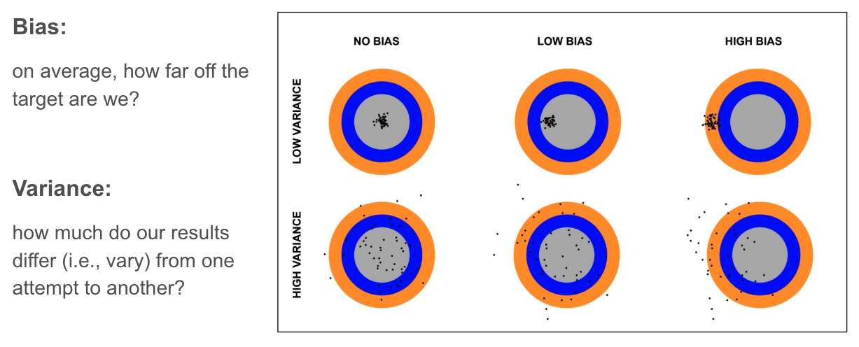
STAT 253 vs STAT 355:
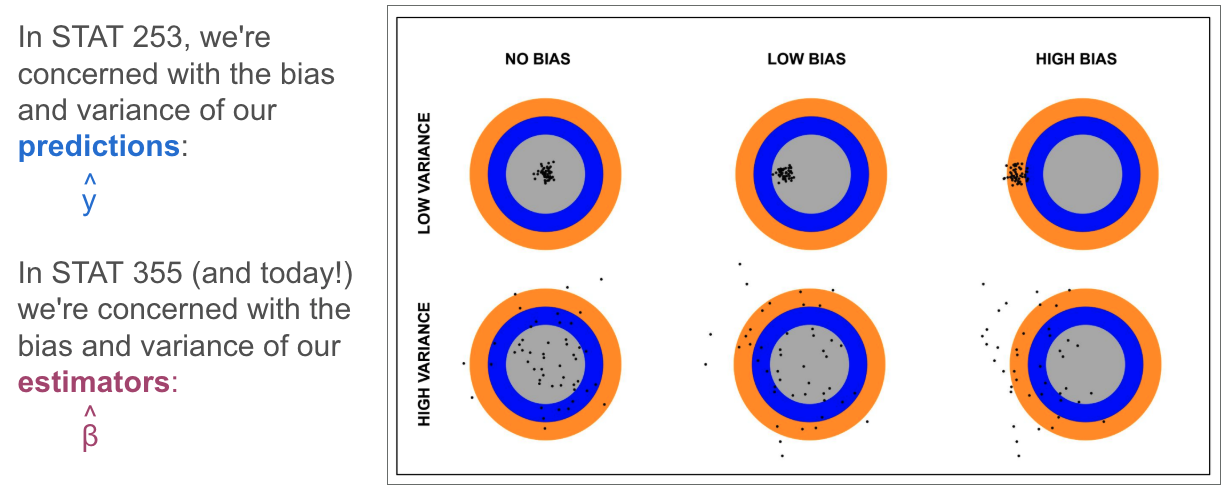
In estimation, just as in prediction, there’s often a bias-variance tradeoff. But, we’ll usually prioritize bias.
Practice Problems
Suppose \(Y_1, \dots, Y_n \stackrel{iid}{\sim} \text{Exponential}(\frac{1}{\theta})\), where \[f_Y(y; \theta) = \frac{1}{\theta} e^{-y/\theta} , \quad y \ge 0.\]
We’ve shown previously that \(\hat\theta_{MLE} = \hat\theta_{MOM} = \frac{1}{n} \sum_{i=1}^n Y_i = \bar{Y}\).
Let’s define \(\hat\theta_1 := \bar{Y}\) and compare this estimator to two other possible estimators of \(\theta\): \(\hat\theta_2 = Y_1\) and \(\hat\theta_3 = n Y_{(1)}\).
Show that all three estimators are unbiased estimators of \(\theta\).
HINT: You can use a Distribution Cheatsheet and the fact that \(Y_{(1)} \sim \text{Exponential}(\frac{n}{\theta})\).
Solution
Let’s start with \(\hat\theta_1\): \[ \begin{aligned} E(\hat\theta_1) &= E(\overline{Y}) \\ & = E(\frac{1}{n}\sum_{i=1}^n Y_i) \\ & = \frac{1}{n}\sum_{i=1}^nE(Y_i), \text{ by linearity of } E() \\ & = \frac{1}{n}\sum_{i=1}^n \theta, \text{ since } Y_i \stackrel{iid}{\sim} \text{Exponential}\left(\frac{1}{\theta}\right) \\ & = \frac{1}{n} n\theta \\ & =\theta, \text{ as desired} \end{aligned} \]
Our other two estimators \(\hat\theta_2, \hat\theta_3\) are also unbiased: \[ \begin{aligned} E(\hat\theta_2) &= E(Y_1) \\ & = \theta, \text{ since } Y_1 \sim \text{Exponential}\left(\frac{1}{\theta}\right) \\ E(\hat\theta_3) & = E(n Y_{(1)}) \\ & = n E(Y_{(1)}) \\ & = n \left(\frac{\theta}{n}\right), \text{ since } Y_{(1)} \sim \text{Exponential}\left(\frac{n}{\theta}\right) \\ & = \theta, \text{ as desired} \end{aligned} \]
We’ll prove that \(Y_{(1)} \sim \text{Exponential}(\frac{n}{\theta})\) below.
Find the variance of \(\hat\theta_1, \hat\theta_2, \hat\theta_3\). Which is most efficient?
Solution
Starting with \(\hat\theta_1\): \[ \begin{aligned} V(\hat\theta_1) &= V(\overline{Y}) \\ & = V\left(\frac{1}{n}\sum_{i=1}^n Y_i\right) \\ & = \left(\frac{1}{n}\right)^2V\left(\sum_{i=1}^nY_i\right) \\ & = \frac{1}{n^2} \sum_{i=1}^n V(Y_i), \text{ since } Y_i \text{ are independent} \\ & = \frac{1}{n^2}\sum_{i=1}^n \theta^2, \text{ since } Y_i \stackrel{iid}{\sim} \text{Exponential}\left(\frac{1}{\theta}\right) \\ & = \frac{1}{n^2} n\theta^2 \\ & = \frac{\theta^2}{n} \end{aligned} \] Then \(\hat\theta_2\): \[ \begin{aligned} V(\hat\theta_2) &= V(Y_1) \\ & = \theta^2, \text{ since } Y_1 \sim \text{Exponential}\left(\frac{1}{\theta}\right) \end{aligned} \] and \(\hat\theta_3\): \[ \begin{aligned} V(\hat\theta_3) & = V(n Y_{(1)}) \\ & = n^2 V(Y_{(1)}) \\ & = n^2 \left(\frac{\theta}{n}\right)^2, \text{ since } Y_{(1)} \sim \text{Exponential}\left(\frac{n}{\theta}\right) \\ & = \theta^2 \end{aligned} \]
From this, we see that \(\hat\theta_1\) is the most efficient (i.e., it has the smallest variance) of the three estimators considered (provided \(n > 1\), which it almost certainly will be; otherwise if \(n = 1\) the estimators are equally efficient).
Find the mean squared error (MSE) of \(\hat\theta_1, \hat\theta_2, \hat\theta_3\), where \[\text{MSE}(\hat\theta) = E\left[(\hat\theta-\theta)^2 \right].\] Which estimator has the smallest MSE?
Solution
The MSE of the first estimator is: \[ \begin{aligned} MSE(\hat\theta_1) &= MSE(\overline{Y}) \\ & = E\left[\left(\overline{Y} - \theta\right)^2 \right] \\ & = E\left[\overline{Y}^2 - 2\overline{Y}\theta + \theta^2 \right] \\ & = E[\overline{Y}^2] - 2\theta E[\overline{Y}] + \theta^2 \\ & = \left(V[\bar{Y}] + E^2[\bar{Y}] \right) - 2\theta \theta + \theta^2 \\ & = \left(\frac{\theta^2}{n} + \theta^2 \right) - \theta^2 \\ & = \frac{\theta^2}{n} \end{aligned} \] and the second: \[ \begin{aligned} MSE(\hat\theta_2) & = MSE(Y_1) \\ & = E[(Y_1 - \theta)^2] \\ & = E[Y_1^2 - 2\theta Y_1 + \theta^2] \\ & = E[Y_1^2] - 2\theta E[Y_1] + \theta^2 \\ & = (V[Y_1] + E^2[Y_1]) - 2\theta\theta + \theta^2 \\ & = (\theta^2 + \theta^2) - \theta^2 \\ & = \theta^2 \end{aligned} \] and the third: \[ \begin{aligned} MSE(\hat\theta_3) & = MSE(nY_{(1)}) \\ & = E[(nY_{(1)} - \theta)^2] \\ & = E[(nY_{(1)})^2 - 2\theta nY_{(1)} + \theta^2] \\ & = E[(nY_{(1)})^2] - 2\theta E[nY_{(1)}] + \theta^2 \\ & = (V[nY_{(1)}] + E^2[nY_{(1)}]) - 2\theta\theta + \theta^2 \\ & = (\theta^2 + \theta^2) - \theta^2 \\ & = \theta^2 \end{aligned} \] So, \(\hat\theta_1\) also has the smallest MSE (unless \(n = 1\), in which case the three estimators have the same MSE).
(MATH/STAT 354 Review) Go back and prove that \(Y_{(1)} \sim \text{Exponential}(\frac{n}{\theta})\). (This will be helpful for PS2!)
HINT: Start by finding the cdf, then the pdf. Review Chapter 1 in the MATH/STAT 355 Notes if you need a refresher.
Solution
To prove that \(Y_{(1)} \sim \text{Exponential}(\frac{n}{\theta})\), we need to find the cdf of \(Y_{(1)}\). Define \(Z := Y_{(1)}\) and let’s find the cdf \(F_Z(z)\)… \[ \begin{aligned} F_Z(z) &= P(Z \le z) \\ & = P(Y_{(1)} \le z) \\ & = 1 - P(Y_{(1)} > z) \\ & = 1 - P(Y_1 > z, \dots, Y_n > z) \\ & = 1 - \prod_{i=1}^n P(Y_i > z), \text{ since } Y_i \text{ are independent} \\ & = 1 - \prod_{i=1}^n [1 - P(Y_i \le z)] \\ & = 1 - \prod_{i=1}^n [1 - F_{Y_i}(z)] \end{aligned} \] But \(F_Y(z)\) is \[ \begin{aligned} F_Y(z) &= P(Y \le z) \\ & = \int_0^z \frac{1}{\theta}e^{-y/\theta} dy \\ & = -e^{-y/\theta}\Big|_0^z \\ & = -e^{-z/\theta} + e^{0} \\ & = 1 - e^{-z/\theta}, \end{aligned} \] So \[ \begin{aligned} F_Z(z) & = 1 - \prod_{i=1}^n [1 - F_{Y_i}(z)] \\ & = 1 - \prod_{i=1}^n [1 - \left(1-e^{-z/\theta} \right)] \\ & = 1 - \prod_{i=1}^n [e^{-z/\theta}] \\ & = 1 - e^{-nz/\theta} \end{aligned} \] From here, we could find the pdf \(f_Z(z)\) using the relationship between the cdf and the pdf: \[ \begin{aligned} f_Z(z) &= \frac{d}{dz} F_Z(z) \\ & = \frac{d}{dz} \left[1 - e^{-nz/\theta} \right] \\ & = -e^{-nz/\theta} (-n/\theta) \\ & = \frac{n}{\theta}e^{-\frac{n}{\theta}z}, \end{aligned} \] which we recognize as the pdf of an Exponential distribution with mean \(\frac{\theta}{n}\), so this tells us that \(Y_{(1)} = Z \sim \text{Exponential}(\frac{n}{\theta})\). Alternatively we could have recognized that \(F_Z(z)\) takes the form of the cdf of an Exponential\(\left(\frac{n}{\theta}\right)\).
(BONUS) In Question 3, you should have found that \(\text{MSE}(\hat\theta) = \text{Var}(\hat\theta)\) for all three estimators. This is not a coincidence! To see why this is happening, prove this general result about the relationship between MSE, variance, and bias: \[\text{MSE}(\hat\theta) = \text{Var}(\hat\theta) + \left[\text{Bias}(\hat\theta)\right]^2.\] Then, use this result to explain what you observed in Question 3.
Solution
The proof is on your problem set this week, so I’ll leave that part up to you 😁
Once we have this result, it is easy to show that the MSE of an unbiased estimator is simply equal to its variance: \[\text{MSE}(\hat\theta) = \text{Var}(\hat\theta) + \text{Bias}^2(\hat\theta) = \text{Var}(\hat\theta) + 0^2 = \text{Var}(\hat\theta)\] Had we known this before, it would have saved us a lot of work in Question 3!
Wrapping Up
After class today, please work on the following: