5  Logistic Regression

Numerical Optimization Techniques for Maximum Likelihood Estimation

Settling In

• Turn in PS1 at the side of the class
  • Is your name on the front page?
  • Did you put a staple in the top left corner?
• Catch up on any recent Slack messages you might have missed
• Review your notes from CP3 and prepare to discuss

Quiz 1

ImportantReminder

Our first quiz is coming up next Friday, February 13!

Content:

• topics: MLE, Least Squares
  • today is the last day of content covered by Quiz 1!
• types of questions:
  • definitions/notation/conceptual understanding (short answer, true/false, multiple choice)
  • derivations
  • no code

Logistics:

• during class time
  • can use the full 60 min, but hopefully won’t take that long!
• closed notes

Questions?

MLE Review

Pull out a piece of paper. Without looking at your notes, answer the following:

1. Using mathematical notation, provide the definition of a maximum likelihood estimate for an unknown parameter \(\theta\).

Solution

In words:

Version 1:

\(\theta_e\) is an maximum likelihood estimate for \(\theta\) if \[L(\theta_e) \ge L(\theta) \quad \forall \theta\]

Version 2:

\[\hat\theta = \arg \max_\theta L(\theta)\]

2. What is the typical procedure for finding an MLE?

Solution

• Find the likelihood \(L(\theta)\)
• Find the log-likelihood \(\log(L(\theta))\)
• Take the derivative of the log-likelihood with respect to \(\theta\)
• Set that derivative equal to zero and solve
• (Recommended: pause and do an intuition check!)

3. Give an example of a scenario where the typical procedure for finding an MLE won’t work.

Solution

The support of the distribution depends on the parameter we are trying to estimate.

Examples:

• \(f_Y(y;\theta) = \frac{1}{\theta}, 0 \le y \le \theta\) (Question 2 on PS1)
• \(f_Y(y) = \frac{2y}{1-\theta^2}, 0 < \theta \leq y \leq 1\) (Question 4 on PS1)

NOTE: The MLE still exists in these scenarios! We just have to use a different process to find it. (NOTE about this NOTE: there are scenarios where the MLE doesn’t exist, this just isn’t one of them)

What do we do instead? Look directly at the likelihood function. Is it monotone increasing (decreasing) over the range of \(\theta\)? If so, we can maximize \(L(\theta)\) by making \(\theta\) as large (small) as possible. Then, check the support of the distribution to see how large/small \(\theta\) can be relative to the observed data.

Logistic Regression

Another example where the “typical” MLE procedure doesn’t work…

Suppose we have a binary outcome variable \(y_i \in \{0, 1\}\), \(i = 1, \dots, n\), and we’re interested in building a model to predict \(y_i\) given information about a predictor variable \(x_i\), \(i = 1, \dots, n\).

We can use logistic regression to do this!

Model Statement/Assumptions

From STAT 155 and STAT 253, you’re probably used to writing a simple logistic regression model as follows: \[\log\left[\text{odds}(y_i = 1 \mid x_i) \right] = \beta_0 + \beta_1 x_i\]

We can re-write this in terms of \(p_i = \text{Pr}(y_i = 1 \mid x_i)\): \[\log\left(\frac{p_i}{1 - p_i} \right) = \beta_0 + \beta_1 x_i\]

If we assume that \(y_i \stackrel{ind}{\sim} \text{Bernoulli}(p_i)\), then we can use MLE to estimate \(\beta_0\) and \(\beta_1\)!

PAUSE: does this seem like a reasonable assumption?

Maximum Likelihood Estimation

Assume \(y_i \sim \text{Bernoulli}(p_i)\), where \(p_i = \frac{\exp(\beta_0 + \beta_1 x_i)}{1 + \exp(\beta_0 + \beta_1 x_i)}\).

Details

\[ \begin{align*} \log\left(\frac{p_i}{1 - p_i} \right) & = \beta_0 + \beta_1 x_i \\ \implies \frac{p_i}{1 - p_i} & = \exp\left( \beta_0 + \beta_1 x_i\right) \\ p_i &= (1-p_i) \exp\left( \beta_0 + \beta_1 x_i\right) \\ p_i & = \exp\left( \beta_0 + \beta_1 x_i\right) - p_i \exp\left( \beta_0 + \beta_1 x_i\right) \\ p_i + p_i \exp\left( \beta_0 + \beta_1 x_i\right) & = \exp\left( \beta_0 + \beta_1 x_i\right) \\ p_i \left(1 + \exp\left( \beta_0 + \beta_1 x_i\right)\right) & = \exp\left( \beta_0 + \beta_1 x_i\right) \\ p_i & = \frac{\exp\left( \beta_0 + \beta_1 x_i\right)}{1 + \exp\left( \beta_0 + \beta_1 x_i\right)} \end{align*} \]

The likelihood is: \[L(\beta_0, \beta_1) = \prod_{i=1}^n \left[ \left(\frac{\exp(\beta_0 + \beta_1 x_i)}{1+\exp(\beta_0 + \beta_1 x_i)} \right)^{y_i} \left(\frac{1}{1+\exp(\beta_0 + \beta_1 x_i)}\right)^{1-y_i}\right]\]

Details

\[ \begin{align*} L(\beta_0, \beta_1) &= \prod_{i=1}^n \left[ p_i^{y_i} (1-p_i)^{1-y_i} \right]\\ & = \prod_{i=1}^n \left[ \left(\frac{\exp(\beta_0 + \beta_1 x_i)}{1+\exp(\beta_0 + \beta_1 x_i)} \right)^{y_i} \left(1 - \frac{\exp(\beta_0 + \beta_1 x_i)}{1+\exp(\beta_0 + \beta_1 x_i)}\right)^{1-y_i}\right] \\ & = \prod_{i=1}^n \left[ \left(\frac{\exp(\beta_0 + \beta_1 x_i)}{1+\exp(\beta_0 + \beta_1 x_i)} \right)^{y_i} \left(\frac{1+\exp(\beta_0 + \beta_1 x_i)}{1+\exp(\beta_0 + \beta_1 x_i)} - \frac{\exp(\beta_0 + \beta_1 x_i)}{1+\exp(\beta_0 + \beta_1 x_i)}\right)^{1-y_i}\right] \\ & = \prod_{i=1}^n \left[ \left(\frac{\exp(\beta_0 + \beta_1 x_i)}{1+\exp(\beta_0 + \beta_1 x_i)} \right)^{y_i} \left(\frac{1}{1+\exp(\beta_0 + \beta_1 x_i)}\right)^{1-y_i}\right] \\ \end{align*} \]

The log likelihood is: \[\log\left[ L(\beta_0, \beta_1) \right] = \sum_{i=1}^n \left(y_i(\beta_0 + \beta_1 x_i) - \log \left[ 1+e^{\beta_0 + \beta_1 x_i}\right] \right)\]

Details

\[ \begin{align*} \log\left[ L(\beta_0, \beta_1) \right] & = \log\left( \prod_{i=1}^n \left[ \left(\frac{\exp(\beta_0 + \beta_1 x_i)}{1+ \exp(\beta_0 + \beta_1 x_i)} \right)^{y_i} \left(\frac{1}{1+\exp(\beta_0 + \beta_1 x_i)}\right)^{1-y_i}\right] \right) \\ & = \sum_{i=1}^n \log \left[ \left(\frac{\exp(\beta_0 + \beta_1 x_i)}{1 + \exp(\beta_0 + \beta_1 x_i)} \right)^{y_i} \left(\frac{1}{1+\exp(\beta_0 + \beta_1 x_i)}\right)^{1-y_i}\right] \\ & = \sum_{i=1}^n \left( \log\left[\left(\frac{\exp(\beta_0 + \beta_1 x_i)}{1+\exp(\beta_0 + \beta_1 x_i)} \right)^{y_i}\right] + \log\left[ \left(\frac{1}{1+\exp(\beta_0 + \beta_1 x_i)}\right)^{1-y_i}\right] \right) \\ & = \sum_{i=1}^n \left(y_i \log \left(\frac{\exp(\beta_0 + \beta_1 x_i)}{1+\exp(\beta_0 + \beta_1 x_i)} \right) + (1-y_i) \log\left(\frac{1}{1+\exp(\beta_0 + \beta_1 x_i)}\right) \right) \\ & = \sum_{i=1}^n \left(y_i \log\left[\exp(\beta_0 + \beta_1 x_i) \right] - y_i \log \left[ 1+\exp(\beta_0 + \beta_1 x_i)\right] -(1 - y_i) \log \left[ 1+\exp(\beta_0 + \beta_1 x_i)\right] \right) \\ & = \sum_{i=1}^n \left(y_i \log\left[\exp(\beta_0 + \beta_1 x_i) \right] - \log \left[ 1+\exp(\beta_0 + \beta_1 x_i)\right] \right) \\ & = \sum_{i=1}^n \left(y_i(\beta_0 + \beta_1 x_i) - \log \left[ 1+\exp(\beta_0 + \beta_1 x_i)\right] \right) \\ \end{align*} \]

The partial derivatives with respect to the unknown parameters are:

\[ \begin{align*} \frac{\partial}{\partial\beta_0} \log[L(\beta_0, \beta_1)] & = \sum_{i=1}^n \left(y_i - \frac{\exp(\beta_0 + \beta_1 x_i)}{1 + \exp(\beta_0 + \beta_1 x_i)} \right) \\ \frac{\partial}{\partial\beta_1} \log[L(\beta_0, \beta_1)] & = \sum_{i=1}^n \left(x_i \left[y_i - \frac{\exp(\beta_0 + \beta_1 x_i)}{1 + \exp(\beta_0 + \beta_1 x_i)}\right] \right) \\ \end{align*} \]

Details

\[ \begin{align*} \frac{\partial}{\partial\beta_0} \log[L(\beta_0, \beta_1)] & = \frac{\partial}{\partial\beta_0} \sum_{i=1}^n \left(y_i(\beta_0 + \beta_1 x_i) - \log \left[ 1+e^{\beta_0 + \beta_1 x_i}\right] \right)\\ & = \sum_{i=1}^n \left(y_i - \frac{1}{1+e^{\beta_0 + \beta_1 x_i}} \left( e^{\beta_0 + \beta_1 x_i}\right) (1) \right) \\ & = \sum_{i=1}^n \left(y_i - \frac{\exp(\beta_0 + \beta_1 x_i)}{1 + \exp(\beta_0 + \beta_1 x_i)} \right) \\ \end{align*} \] and \[ \begin{align*} \frac{\partial}{\partial\beta_1} \log[L(\beta_0, \beta_1)] & = \frac{\partial}{\partial\beta_1} \sum_{i=1}^n \left(y_i(\beta_0 + \beta_1 x_i) - \log \left[ 1+e^{\beta_0 + \beta_1 x_i}\right] \right)\\ & = \sum_{i=1}^n \left(y_i x_i - \frac{1}{1+e^{\beta_0 + \beta_1 x_i}} \left( e^{\beta_0 + \beta_1 x_i}\right) (x_i) \right) \\ & = \sum_{i=1}^n \left(x_i \left[y_i - \frac{\exp(\beta_0 + \beta_1 x_i)}{1 + \exp(\beta_0 + \beta_1 x_i)} \right]\right) \\ \end{align*} \]

If we set these partial derivatives equal to zero and try to solve that system of equations, we get stuck: there’s no closed form solution. Enter: numerical optimization techniques.

Numerical Optimization Techniques

One technique we can use to solve for \(\beta_0, \beta_1\) is known as Fisher Scoring, named after the famous statistician, Ronald Fisher (we’ll see his name a few more times this semester!).

Fisher Scoring is just a variation on the Newton-Raphson method, a general root-finding algorithm that you may have seen in Calculus!

Newton-Raphson

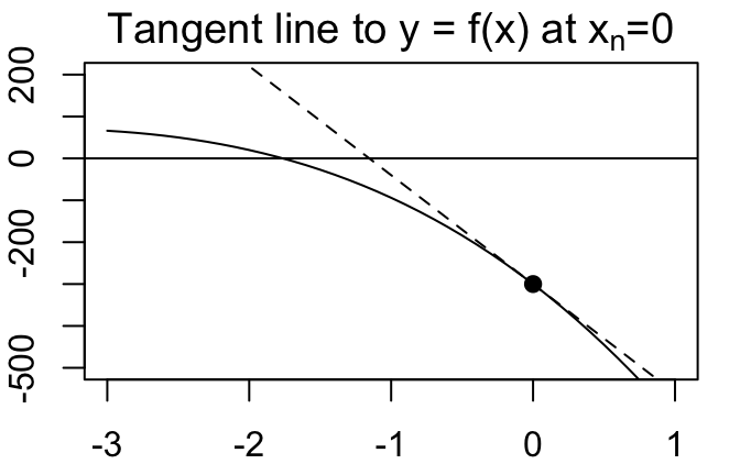
Suppose we want to find the root of \(f(x)\). In other words, we want to know the value of \(x\) for which \(f(x) = 0\).

To find the root, Newton-Raphson tells us to do the following:

1. Start with an initial guess \(x^{(0)}\) (eg \(x^{(0)} = 0\) in the image below)
2. Update the guess according to \(x^{(1)} = x^{(0)} - f(x^{(0)}) / f'(x^{(0)})\)
3. Continue updating \(x^{(t+1)} = x^{(t)} - f(x^{(t)}) / f'(x^{(t)})\), \(t = 1, 2, ...\) until you converge on a solution

Fisher Scoring

Maximum Likelihood Estimation is a root-finding problem! We want to find the value of \(\theta\) for which \(\frac{\partial}{\partial \theta} \log(L(\theta)) = 0\).

We often refer to \(\frac{\partial}{\partial \theta} \log(L(\theta))\) as the score, \(S(\theta)\). Hence the name: Fisher Scoring!

If we want to use Newton-Raphson to find the MLE for an unknown parameter \(\theta\), the steps are thus:

1. Start with an initial guess \(\theta^{(0)}\).
2. Update the guess: \(\theta^{(1)} = \theta^{(0)} - S(\theta^{(0)})/S'(\theta^{(0)})\)
3. Continue updating \(\theta^{(t+1)} = \theta^{(t)} - S(\theta^{(t)})/S'(\theta^{(t)})\), \(t = 1, 2, ...\) until you converge on a solution

If we have multiple unknown parameters, \(\theta_1, \theta_2, \dots, \theta_p\), this becomes:

1. Start with initial guesses for each parameter: \(\boldsymbol\theta^{(0)}\)

2. Update the guesses: \(\boldsymbol\theta^{(1)} = \boldsymbol\theta^{(0)} - S(\boldsymbol\theta^{(0)})/S'(\boldsymbol\theta^{(0)})\)

3. Continue updating \(\boldsymbol\theta^{(t+1)} = \boldsymbol\theta^{(t)} - S(\boldsymbol\theta^{(t)})/S'(\boldsymbol\theta^{(t)})\), \(t = 1, 2, ...\) until you converge on a solution

where \(\boldsymbol\theta = \begin{bmatrix} \theta_1 \\ \theta_2 \\ \vdots \\ \theta_p \end{bmatrix}\),

\[ S(\boldsymbol\theta) = \frac{\partial}{\partial \boldsymbol\theta} \log\left[ L(\boldsymbol\theta) \right] = \begin{bmatrix} \frac{\partial}{\partial\theta_1}\log\left[ L(\theta_1, \dots, \theta_0) \right] \\ \frac{\partial}{\partial\theta_2}\log\left[ L(\theta_1, \dots, \theta_0) \right] \\ \vdots \\ \frac{\partial}{\partial\theta_p}\log\left[ L(\theta_1, \dots, \theta_0) \right] \end{bmatrix} \]

and \[ S'(\boldsymbol\theta) = \frac{\partial}{\partial \boldsymbol\theta} S(\boldsymbol\theta) = \begin{bmatrix} \frac{\partial^2}{\partial\theta_1 \partial\theta_1}\log\left[ L(\theta_1, \dots, \theta_0) \right] & \dots & \frac{\partial^2}{\partial\theta_1 \partial\theta_p}\log\left[ L(\theta_1, \dots, \theta_0) \right] \\ \frac{\partial^2}{\partial\theta_2 \partial\theta_1}\log\left[ L(\theta_1, \dots, \theta_0) \right] & \dots & \frac{\partial^2}{\partial\theta_2 \partial\theta_p}\log\left[ L(\theta_1, \dots, \theta_0) \right] \\ \vdots & \ddots & \vdots \\ \frac{\partial^2}{\partial\theta_p \partial\theta_1}\log\left[ L(\theta_1, \dots, \theta_0) \right] & \dots & \frac{\partial^2}{\partial\theta_p \partial\theta_p}\log\left[ L(\theta_1, \dots, \theta_0) \right] \end{bmatrix} \]

Exercises

Open RStudio and create a new Quarto document so you have somewhere to record your work.

Scenario: Suppose \(X_1, X_2, \dots, X_n\) are a random sample from the Exponential pdf with parameter \(\lambda > 0\): \[f_X(x; \lambda) = \lambda e^{-\lambda x}, \quad x \ge 0\]

Let’s use the Newton-Raphson Method to find the maximum likelihood estimate for \(\lambda\), if a random sample of size 5 yielded the following measurements:

[1] 0.854 1.911 0.014 0.632 1.286

1. First, derive the likelihood, log likelihood, score, and first derivative of the score. (Check your answers with your neighbors and Kelsey before you move on to the next step!)

Solution

\[ \begin{align*} L(\lambda) & = \prod_{i=1}^n \lambda e^{-\lambda y_i} \\ & = \lambda^n e^{- \lambda \sum y_i} \\ \log(L(\lambda)) & = n \log \lambda - \lambda \sum y_i \\ S(\lambda) & = \frac{\partial}{\partial \lambda} \log(L(\lambda)) \\ & = \frac{n}{\lambda} - \sum y_i \\ S'(\lambda) & = \frac{\partial}{\partial \lambda} S(\lambda) \\ & = -n \lambda^{-2} \end{align*} \]

2. Next, define some functions in R that will evaluate the score and first derivative of the score for a given \(\lambda\) and sample of observed values (\(\mathbf{x} = x_1, x_2, ..., x_n\)). I did the first one for you. You finish the second!

# score function
S <- function(lambda, y){
  length(y)/lambda - sum(y)
}  

# first derivative of score function 
Sprime <- function(lambda, y){
  # your code here
}

Solution

# score function
S <- function(lambda, y){
  length(y)/lambda - sum(y)
}  

# first derivative of score function
Sprime <- function(lambda, y){
  -length(y) / (lambda^2)
}

 

3. Using a starting value of \(\lambda^{(0)} = 0.5\), step through the Newton-Raphson process until you converge on a stable estimate for \(\lambda\). (Hint: it should take about 6 steps.)

# store data in vector
example_data <- c(0.854, 1.911, 0.014, 0.632, 1.286)

# starting value
lambda_0 <- 0.5

# first update
lambda_1 <- ___

# second update 
lambda_2 <- ___

# etc. 

Solution

# store data in vector
example_data <- c(0.854, 1.911, 0.014, 0.632, 1.286)

# starting value
lambda_0 <- 0.5

# first update
lambda_1 <- lambda_0 - S(lambda_0, example_data)/Sprime(lambda_0, example_data)
print(lambda_1)

[1] 0.76515

# second update 
lambda_2 <- lambda_1 - S(lambda_1, example_data)/Sprime(lambda_1, example_data)
print(lambda_2)

[1] 0.980324

# third update
(lambda_3 <- lambda_2 - S(lambda_2, example_data)/Sprime(lambda_2, example_data))

[1] 1.057852

# fourth update
(lambda_4 <- lambda_3 - S(lambda_3, example_data)/Sprime(lambda_3, example_data))

[1] 1.064468

# fifth update
(lambda_5 <- lambda_4 - S(lambda_4, example_data)/Sprime(lambda_4, example_data))

[1] 1.064509

# sixth update
(lambda_6 <- lambda_5 - S(lambda_5, example_data)/Sprime(lambda_5, example_data))

[1] 1.064509

# seventh update
(lambda_7 <- lambda_6 - S(lambda_6, example_data)/Sprime(lambda_6, example_data))

[1] 1.064509

Suggestion: can you write a for loop or something similar to iterate through these steps in a more efficient way?

4. Compare your solution from Newton-Raphson to the MLE you derived “by hand” on PS1. Are they the same? (Hint: they should be!)

Solution

On PS1, we found that \(\hat\lambda_{MLE} = \frac{n}{\sum_{i=1}^n x_i} = \left(\bar{x}\right)^{-1}\). Plugging in our observed data, we get

1/mean(example_data)

[1] 1.064509

This is the same as our Newton-Raphson estimate from Question 3: 1.0645093.

5. Try Newton-Raphson again using different starting values. Do you ever get a different answer?

Solutions

The Newton-Raphson method can be sensitive to starting values, so in practice it’s useful to try several different starting values to see what happens. When choosing a starting value, make sure to pay attention to any bounds on the parameter value. In this example, we know \(\lambda\) should be greater than 0, so we should only use positive starting values. Note that changing the starting value can also change how many steps it takes for the Newton-Raphson Method to converge.

Going Deeper

Finished with the exercises above? Try one of the following challenge/bonus exercises:

Logistic Regression

See how far you can get in setting up the Fisher Scoring approach for a simple logistic regression model. You can use the likelihood, log likelihood, and score functions given above as a starting point.

EM Algorithm

Read about the Expectation-Maximization (EM) Algorithm, another computational technique that’s used to find MLEs.

Here’s one resource to get you started: Peng (2022) [link].

Wrapping Up

After class today, please:

• Re-organize and review your notes to help deepen your understanding, solidify your learning, and make homework go more smoothly!
• Complete CP4 (Method of Moments) before next class.
• Start studying for Quiz 1!

Peng, Roger D. 2022. Advanced Statistical Computing.