8 Simulations

Using Monte Carlo simulations to assess estimator properties

Settling In

Sit somewhere new:
- Find people whose first name starts with the same letter as you (i.e., arrange yourselves alphabetically!)
- Introduce yourselves / check in with each other
Catch up on any recent Slack messages you might have missed
Reminder: PS2 due Friday
- Let me know in advance if you need an extension.

Activity: Using Simulations to Compare Estimators

Let’s review estimation techniques (MLE, MOM) and estimator properties (bias, variance). We’ll also see how we can use simulations to assess estimator properties when we can’t (or don’t want to) do those calculations by hand.

Open RStudio and create a new Quarto document so you have somewhere to record your work.

The Scenario

Kelsey wants to go the 2026 World Cup ⚽️.

She recently entered a ticket lottery and is waiting to hear the results. In the meantime, she wants to estimate how many other people applied, and thus have a better sense of her chance of getting tickets.

Here’s some info we’ll use to figure this out:

Each person that enters the ticket lottery is given an application number, in order of when they applied: the first person to apply gets application number 1, the second gets application number 2, etc.

(In case you’re curious: Kelsey’s application number is 26194987.)
Let \(\theta\) represent the final applicant (and thus, also, the total number of applicants). This is what we want to estimate.
Assuming each entry has an equal chance of selection, we can represent the chance that an application is selected with the (discrete) Uniform distribution from 1 to \(\theta\): \[f_X(x; \theta) = \frac{1}{\theta}, \quad x = 1, ..., \theta.\]

Our question: Given some data points (application numbers), how can we estimate \(\theta\)?

Note

This is very similar to the \(\text{Unif}(0, \theta)\) scenario we’ve been considering in recent classes and problem sets. We’re just looking at a discrete random variable here instead of continuous.

Part 1: Estimation (Review)

Let’s consider three possible estimators of \(\theta\):

The maximum likelihood estimator, \(\hat\theta_1 = X_{(n)}\), the \(n\)th order statistic / sample maximum.
The method of moments estimator, \(\hat\theta_2 = 2 \bar{X} - 1\).

A third estimator, \(\hat\theta_3 = \frac{n+1}{n}X_{(n)} - 1\).
- We’ll talk about where this comes from later. For now, just trust me that it’s a “reasonable” estimator of \(\theta\).

Your first task is this…

Confirm that the MLE and MOM estimators for \(\theta\) are \(X_{(n)}\) and \(2 \bar{X} - 1\), as stated above.

HINT: \(\sum_{k=1}^n k = \frac{n(n+1)}{2}\).

Solution

To find the MLE, we need to look at the likelihood: \[L(\theta) = \prod_{i=1}^n f_X(x_i; \theta) = \prod_{i=1}^n \frac{1}{\theta} = \theta^{-n}.\] Just as in the continuous uniform case, notice that the support of our pdf depends on the unknown parameter, \(\theta\), that we are trying to estimate. (So, our MLE will be an order statistic.) Notice that \(L(\theta)\) is monotone decreasing in \(\theta\): as \(\theta\) gets bigger, \(\frac{1}{\theta}\) gets smaller, and thus so too does \(\left(\frac{1}{\theta}\right)^n\). Thus, to maximize \(L(\theta)\) we need to make \(\theta\) as small as possible. But the smallest \(\theta\) can be is \(X_{\max} = X_{(n)}\) (since \(\theta \ge X_i \forall i\)). So, our MLE is \(\hat\theta_{MLE} = X_{(n)}\).

To find the method of moments estimator for \(\theta\), we need to know the first moment of our discrete uniform distribution. We can find this using the definition of the expected value of a discrete random variable: \[\begin{align*} E(X) & = \sum_{x = 1}^\theta x f_X(x; \theta) \\ & = \sum_{x = 1}^\theta x \frac{1}{\theta} \\ & = \frac{1}{\theta} \sum_{x = 1}^\theta x \\ & = \frac{1}{\theta} \frac{\theta (\theta+1)}{2} \\ & = \frac{\theta+1}{2} \end{align*}\]

Part 2: Bias

In comparing these three estimators, one of the first properties to consider is bias. Two of the estimators proposed above are unbiased estimators of \(\theta\), and one is biased.

Provide an intuitive argument as to why \(\hat\theta_1\) is a biased estimator for \(\theta_1\).

Solution

Note that \(\theta \ge X_i \ \forall i\), ie \(\theta\) is an upper bound for our \(X_i\)s. Thus, \(X_{(n)}\), the largest of our observations, will either be equal to \(\theta\) or smaller than it — but never larger! In other words, the estimator \(\hat\theta_1 = X_{(n)}\) will always underestimate \(\theta\): the expected value of \(X_{(n)}\) will be some number smaller than \(\theta\).
Show that the MOM estimator, \(\hat\theta_2\), is an unbiased estimator for \(\theta\).

Solution

We must show \(E(\hat\theta_2) = \theta\). Well, \[\begin{align*} E(\hat\theta_2) & = E(2 \bar{X} - 1) \\ & = 2 E(\bar{X}) - 1 \\ & = 2 E\left(\frac{1}{n}\sum_{i=1}^n X_i \right) - 1 \\ & = 2 \frac{1}{n}\sum_{i=1}^n E(X_i) - 1 \\ & = \frac{2}{n} \sum_{i=1}^n \left(\frac{\theta+1}{2}\right) - 1 \\ & = \frac{2}{n} n \left(\frac{\theta+1}{2}\right) - 1 \\ & = \theta + 1 - 1 \\ & = \theta, \end{align*}\] as desired.
The third estimator, \(\hat\theta_3\) is also an unbiased estimator for \(\theta\). If you wanted to prove this, what would you need to do? Sketch out the steps. (No need to actually perform those steps!)

Solution

To show \(\hat\theta_3\) is an unbiased estimator for \(\theta\), we need to show that \(E(\hat\theta_3) = \theta\). Thus, we need to know the expected value of \(\hat\theta_3 = \frac{n+1}{n}X_{(n)} - 1\). We know that \[E\left( \frac{n+1}{n}X_{(n)} - 1\right) = \frac{n+1}{n} E(X_{(n)}) - 1.\] But what is \(E(X_{(n)})\)?

Note that \(X_{(n)}\) does not have the same distribution as the observations \(X_1, ..., X_n \sim \text{DiscreteUniform}(1, \theta)\). The sample maximum, \(X_{(n)}\) is the largest of \(n\) observations from this discrete uniform distribution. Although the chance that any one observation \(X_i = 1\) is \(\frac{1}{\theta}\), it is much less likely that \(X_{(n)} = 1\). (For this to happen, we would have needed to get \(X_1 = 1, X_2 = 1, \dots, X_n = 1\) — unlikely.) Our task is to find the distribution of the random variable \(Z \equiv X_{(n)}\). Once we know the pmf, we can find the expected value using its definition \(E(Z) = \sum_{z} z f_Z(z)\).

We did something like this in the Bias and Variance exercises, except with \(X_{(1)}\) instead of \(X_{(n)}\). It helps to start by finding the CDF \(F_Z(z) = \Pr(Z \le z)\). If you know \(Z = X_{(n)} \le z\), what do you know about \(X_1, X_2, \dots, X_n\)? Once you find the CDF, how can you find the PDF?

It is possible, but annoying, to analytically derive the bias of \(\hat\theta_1\) and \(\hat\theta_3\) in this discrete uniform context. Instead, let’s use simulations to learn more about these estimators’ behavior.

Note

We got through Part 2 on Day 1 (Feb 18) and will finish the rest on Day 2 (Feb 20). If you missed Day 1, please work through Parts 1 and 2 on your own and come to our next class prepared to work on Parts 3+.

Part 3: Simulations

Background: Simulation Studies

Simulation studies are a widely used technique in statistical research. The general idea is this…

We “simulate”, or artificially generate, data in a way where we know the “truth”. Then, we apply a statistical method to these simulated data to see how it performs. Since we created the data, we can compare the result we get from our statistical method to the “truth” and get a sense of how accurate the method is.

This is a particularly useful framework when we want to evaluate a new method, understand how a method’s performance varies across different scenarios, or compare multiple methods against each other. It can also be useful in contexts (like Kelsey’s research area of statistical genetics) in which finding/working with “real” data can be challenging due to data privacy concerns, logistical constraints, etc.

Let’s apply this framework to our problem of assessing the bias of our three estimators \(\hat\theta_1, \hat\theta_2, \hat\theta_3\).

STEP 1: Simulate Data.

First, we need to simulate some data. Recall that we are assuming our data come from a discrete Uniform distribution from 1 to \(\theta\), where each value between 1 and \(\theta\) has an equal chance of being selected. If we specify the “true” value of \(\theta\), we can then use the sample function in R to generate data from this distribution.

# set seed for reproducibility
set.seed(355) 

# generate one data point from discrete unif (1,100)
sample(1:100, size = 1)

[1] 69

If we want to repeat this process \(n\) times (replicating the idea of observing a random sample \(X_1, \dots, X_n\) from this distribution), we update our code slightly:

# set seed for reproducibility
set.seed(355) 

# generate 10 data points from a discrete unif
sample(1:100, size = 10, replace = T)

 [1]  69   3  49  52   8 100  16  86  53  76

Why did we need to add the replace = T argument to the sample function, above?

Solution

We need to sample with replacement in order for the observations to be sampled independently from this distribution.

To perform a simulation study, we will ultimately want to generate many datasets of varying sizes, with different choices of \(\theta\), etc. To save ourselves some typing (or copy-pasting) later, let’s write our own R function that takes in values of \(\theta\) and \(n\) and returns a vector of \(n\) data points independently sampled from a discrete uniform distribution from 1 to \(\theta\).

generate_data <- function(theta, n){
  sample(1:theta, size = n, replace = T)
}

Try running this function with a few different values of theta, n, and seeds to confirm it’s working the way you expect.

set.seed(355)
generate_data(theta = 100, n = 10)

set.seed(1)
generate_data(theta = 100, n = 10)

set.seed(355)
generate_data(theta = 20, n = 5)

# etc.

Solution

# random sample of size 10 from a DiscreteUniform(1, 100)
set.seed(355)
generate_data(theta = 100, n = 10)

 [1]  69   3  49  52   8 100  16  86  53  76

# another random sample of size 10 from a DiscreteUniform(1, 100) 
set.seed(1)
generate_data(theta = 100, n = 10)

 [1] 68 39  1 34 87 43 14 82 59 51

# random sample of size 5 from a DiscreteUniform(1, 20)
set.seed(355)
generate_data(theta = 20, n = 5)

[1]  5 13 13  3 17

# etc.

STEP 2: Calculate Estimates.

Now that we can generate simulated data, the next step is to apply our methods (estimators) to these data and see how they perform.

Let’s write functions in R that take in a vector of data points (x = c(x_1, x_2, ..., x_n)) and return estimates for \(\hat\theta_1\), \(\hat\theta_2\), and \(\hat\theta_3\). I did the first one for you. Finish the other two.

estimate1 <- function(x){
  max(x)
}

estimate2 <- function(x){
  # your code here  
}

estimate3 <- function(x){
  # your code here  
}

Solution

estimate1 <- function(x){
  max(x)
}

estimate2 <- function(x){
  2*mean(x) - 1
}

estimate3 <- function(x){
  n <- length(x)
  ((n+1)/n)*max(x) - 1
}

Test your functions on a simulated datasets to confirm they’re working the way you expect. Fix your code if not.

# generate data
set.seed(355)
test_data <- generate_data(theta = 100, n = 10)

# check estimates
estimate1(test_data)
estimate2(test_data)
estimate3(test_data)

Solution

# generate data
set.seed(355)
test_data <- generate_data(theta = 100, n = 10)

# look at data
print(test_data)

 [1]  69   3  49  52   8 100  16  86  53  76

mean(test_data) # sample mean

[1] 51.2

# check estimates
estimate1(test_data) # sample max = 100

[1] 100

estimate2(test_data) # 2 * 51.2 - 1 = 101.4

[1] 101.4

estimate3(test_data) # (11/10)* sample max - 1 = 109

[1] 109

On this “test” data, which estimate was closest to the true value of \(\theta\)?

Solution

\(\hat\theta_1\) was closest to the truth in this dataset. We got a bit lucky here and actually sampled the true maximum \(\theta = 100\).

STEP 3: Repeat.

From this last question, we are starting to get a sense of the bias of our estimators. But, we don’t want to draw any strong conclusions based on just a single test dataset. If we had gotten a different random sample, would the same estimator look best? Let’s repeat this process many times and see what happens!

To help with this, let’s write a function that combines our steps from earlier: (1) generate data and (2) calculate all three estimates on those data.

do_one_sim <- function(theta, n){
  # get data
  sim_data <- generate_data(theta = theta, n = n)
  
  # get estimates
  t1 <- estimate1(sim_data)
  t2 <- estimate2(sim_data)
  t3 <- estimate3(sim_data)
  
  # combine estimates into one vector 
  sim_results <- c(theta1 = t1, theta2 = t2, theta3 = t3)
  return(sim_results)
}

Run the do_one_sim function a few times to confirm you understand what it’s doing.

Solution

# this should match what we did above
set.seed(355)
do_one_sim(theta = 100, n = 10)

theta1 theta2 theta3 
 100.0  101.4  109.0

# try with a different seed
# (notice that the first estimator is not as good this time!)
set.seed(1)
do_one_sim(theta = 100, n = 10)

theta1 theta2 theta3 
  87.0   94.6   94.7

Now that we’ve set up this function to do a single run-through of our simulation, we can use the replicate function in R to repeat/replicate this many times.

# repeat simulation 1000 times
# using theta = 100, n = 10
set.seed(355)
sim_results <- replicate(n = 1000, do_one_sim(theta = 100, n = 10))

# look at first 5 reps
sim_results[,1:5]

        [,1]  [,2]  [,3] [,4]  [,5]
theta1 100.0  98.0  95.0 88.0  98.0
theta2 101.4 111.6 113.2 85.4 112.6
theta3 109.0 106.8 103.5 95.8 106.8

(OPTIONAL) If you’ve taken COMP/STAT 212 or have other R programming experience, do you have any other ideas of how to run the do_one_sim function 1000 times (and store all the resulting estimates), using some approach other than the replicate() function?
Solution

Here are a few ideas (not an exhaustive list!):
- for loop (probably not more efficient, though — R is notoriously slow at for loops)
- map() functions in the purrr package (link)

Create a visualization that compares the distribution of estimates from each estimator across the 1000 simulation replicates.

Solution

Here’s one way to visualize our results:

# do some data wrangling to make this easier to plot
library(tidyverse)
sim_data <- sim_results %>%
  t() %>%
  as.data.frame() %>%
  pivot_longer(cols = starts_with('theta'), names_to = 'estimator')

# density plots
sim_data %>%
  ggplot(aes(x = value, fill = estimator)) + 
  geom_density(alpha = 0.5) + 
  geom_vline(xintercept = 100, linetype = 2, size = 1.2) + 
  theme_bw()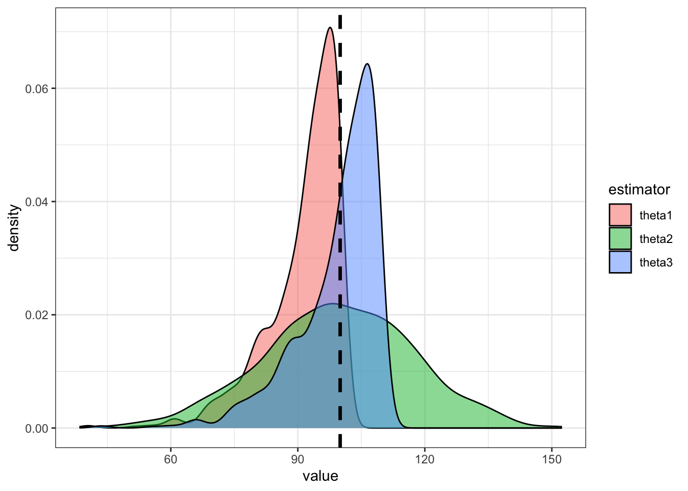

Notice that the estimates from \(\hat\theta_2\) and \(\hat\theta_3\) are centered in the right spot (around the true \(\theta = 100\)), but the estimates from our MLE tend to be too small.

Calculate the empirical bias of your estimators: subtract the true value of theta from the average (across the 1000 simulation replicates) of each set of estimates. Which estimator(s) have the smallest bias?
Solution
# empirical bias of estimator 1 mean(sim_results[1,]) - 100
```
[1] -8.767
```
# empirical bias of estimator 2 mean(sim_results[2,]) - 100
```
[1] -0.6828
```
# empirical bias of estimator 3 mean(sim_results[3,]) - 100
```
[1] -0.6437
```
\(\hat\theta_3\) and \(\hat\theta_2\) both have empiricial bias close to zero

Part 4: Variance

We’ve focused on the bias of our estimators thus far. In this case, we have two unbiased estimators: \(\hat\theta_2\) and \(\hat\theta_3\). To decide between them, let’s look at their variance!

Based on your simulation study above, which estimator has the lowest variance?
Solution

We can see pretty clearly from the density plots above that \(\hat\theta_3\) has lower variance than \(\hat\theta_2\). We can confirm this empirically:
# empirical variance of estimator 2 var(sim_results[2,])
```
[1] 317.7417
```
# empirical variance of estimator 3 var(sim_results[3,])
```
[1] 91.56116
```

Combining all of the information about these estimators, which do you think is “best”? Why?
Solution

\(\hat\theta_3\) is the best of the three estimators we considered here! It is unbiased and has smaller variance than the other unbiased estimator, \(\hat\theta_3\).

Notice that \(\hat\theta_1\) actually has the smallest variance of the three, but it is biased – which we don’t love. I’d still stick with \(\hat\theta_3\).
var(sim_results[1,])
```
[1] 75.67038
```
One question you might be asking yourself is this: \(\hat\theta_3\) is the “best” estimator of the three we considered, but can we do any better? It turns out, in this scenario, we cannot. \(\hat\theta_3\) is what’s known as a uniformly minimum variance unbiased estimator (UMVUE), which means that among all possible unbiased estimators of \(\theta\) it has the smallest variance. We’ll talk about how to prove this and how to construct UMVUEs in the next few weeks of class!

Part 5: Back to the World Cup…

Use your favorite estimator to give Kelsey an estimate of the total number of World Cup ticket applications.

Here’s the (very small, and not actually “random”) sample that she has:

\(X_1\) = 26194987
\(X_2\) = 26185749
\(X_3\) = 26190381
\(X_4\) = 27364827
if you applied for tickets, add your own data :)

Solutions

# set up data
worldcup_data <- c(26194987,26185749,26190381,27364827)

# estimate the total number of applications using our UMVUE
estimate3(worldcup_data)

[1] 34206033

# out of curiosity, let's see what the other estimators give us too
estimate1(worldcup_data)

[1] 27364827

estimate2(worldcup_data)

[1] 52967971

It turns out that our estimates are too low, at least based on the data I gave you. According to a recent New York Times article, over 500 million people (!!!) applied for tickets: (source).

I guess that explains why my ticket application was unsuccessful 😭😭😭

Going Deeper

Finished with the exercises above?

Repeat the simulation study with a few different values of \(\theta\). What do you notice?
Repeat the simulation study with different sample sizes. What do you notice?

NOTE: This question relates to the idea of studying asymptotic properties of estimators. We’ll talk more about this soon!
Derive the bias and variance of the three estimators analytically.
Google the “German Tank Problem.” How is it similar to the scenario we considered today?
Check out this example of a research paper that uses simulations to compare methods: Grinde et al. (2019) [link]

Wrapping Up

Reminders about some upcoming deadlines:

PS2: Feb 20 (in class)
CP6: Feb 23 (before class)
Quiz 1 Revisions: stop by office hours before the next quiz
Quiz 2: Feb 27 (in class)

Grinde, Kelsey E, Lisa A Brown, Alexander P Reiner, Timothy A Thornton, and Sharon R Browning. 2019. “Genome-Wide Significance Thresholds for Admixture Mapping Studies.” The American Journal of Human Genetics 104 (3): 454–65.