introduce yourselves: name, pronouns, class year, major, hometown, highlights from your winter break, something you’re looking forward to this semester (in Stat Theory or otherwise!), etc.
check in with each other
brainstorm a list of statistical techniques or concepts that you’ve come across in previous courses where the underlying mathematical details were simplified or skipped altogether. which are you particularly curious to learn more about?
Meet Your Instructor
Name: call me “Kelsey” or “Professor Grinde”
Pronouns: she/her/hers
Hometown(s):
Plymouth, MN (\(\approx\) 20 years)
St. Paul, MN (6.5 years)
Major(s):
BA in Math @ St. Olaf College
PhD in Biostatistics @ University of Washington
Things I love about Stat Theory:
Familiar faces 😁
Putting the pieces of your major together (math prereqs + stat methods)
Learning the “why” behind concepts you’ve seen before
Great prep for grad school
This was one of the most formative classes I took as a student!
Some other things I love (not necessarily in this order!):
Syllabus Highlights
Course Overview
In this course we will…
build a deeper understanding of methods you’ve come across in earlier statistics courses by exploring their mathematical underpinnings
develop skills that will be useful for future study/work in statistics (writing proofs, conducting simulation studies, typesetting in LaTeX, etc.)
see topics that are often covered in graduate-level statistics courses
Note
This course will has a different feel and focus than other stats classes you’ve taken at Mac! We will do a lot of math, some computation, and almost no data application.
Small Group Discussion
At your table, discuss:
What’s one thing you’re good at outside of school?
How did you get good at that thing?
Once you’ve discussed as a table, share (and upvote) responses to Question #2 here:
Course Structure
This is a challenging course. To help support you in that challenge, we will:
Devote a lot of class time to practice.
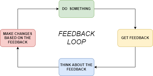
Have lots of opportunities to engage in feedback loops.
Devote a lot of class time to practice –> partially flipped classroom
before some (but not all) classes: watch videos, read, complete corresponding “checkpoint” quizzes
during class time: work on practice problems in small groups
Have lots of opportunities to engage in feedback loops –> “standards-based” testing
quizzes approx. every other week
for each topic, you’ll get a score of pass, revise, or retake
revise –> reattempt during office hours
retake –> try again on the next quiz (same concept, new question)
final quiz grade determined by the proportion of topics that you pass by the 2nd attempt
Questions about this or anything else on the Syllabus?
Least Squares Estimation
The first part of this course will focus on the topic of estimation, exploring different techniques for estimating the value of unknown parameters in probability models.
You’re already familiar with one such technique—least squares estimation—from STAT 155 and STAT 253.
Motivating Example
Forced expiratory volume (FEV) is a measure of lung capacity. Higher values indicate higher lung capacity—the ability to blow out more air in one second—and therefore indicate better lung function.
The fev.csv dataset contains data on lung function for a total of 654 children, ages 3-19. Each row in the dataset corresponds to a single child’s visit to a doctor’s clinic. All children participating in this study attended the same pediatric clinic. The exact date of the study is unknown, but we at least know that it took place before 2005. Variables collected include:
age at time of measurement (years)
measured forced expiratory volume fev (liters per second)
height at time of measurement (inches)
binary sex (male/female)
indicator of smoking habits smoke (smoker/nonsmoker)
head(fev)
  subjid age   fev height    sex     smoke
1    301   9 1.708   57.0   male nonsmoker
2    451   8 1.724   67.5   male nonsmoker
3    501   7 1.720   54.5   male nonsmoker
4    642   9 1.558   53.0 female nonsmoker
5    901   9 1.895   57.0 female nonsmoker
6   1701   8 2.336   61.0   male nonsmoker
Suppose we wanted to understand the relationship between height and lung function. We could do this by fitting a simple linear regression model
where fev is our outcome and height is our explanatory variable.
We can fit this model in R by running the code below:
model1 <-lm(fev ~ height, data = fev)coef(model1)
(Intercept)      height
 -5.4326788   0.1319756
As you learned in STAT 155 and STAT 253, R is using least squares estimation to estimate the intercept (\(\hat\beta_0\) = -5.43) and slope (\(\hat\beta_1\) = 0.13).
In the rest of this activity, you’ll derive the least squares estimates by hand!
Review: Least Squares Estimation
In fitting this simple linear regression model, our goal is to find the line that provides the “best” fit to our data.
More specifically, we hope to find the values of the intercept \(\beta_0\) and slope \(\beta_1\) that minimize the sum of squared residuals:
In order to find the least squares estimates for the intercept and slope of our simple linear regression model, we need to minimize a function (the sum of squared residuals).
To do this, we can use techniques from multivariable calculus!
If we want to find the value of \(x\) that minimizes the function \(f(x)\), then we need to…
take the derivative \(f'(x) = \frac{d}{dx} f(x)\)
set the derivative equal to zero and solve for \(x\)
find the second derivative \(f''(x)\), evaluate at the solution to step #2, and check if it’s positive in order to confirm we have a minimum
(we should also check the endpoints!)
Exercises
To find the least squares estimates \(\hat\beta_0, \hat\beta_1\), we start by finding the partial derivatives \(\frac{\partial}{\partial\beta_0}\) and \(\frac{\partial}{\partial\beta_1}\) of the sum of squared residuals.
From here, we can plug our slope estimate \(\hat\beta_1\) back into the equation for \(\beta_0\) above to get our estimate for the intercept \[\hat\beta_0 = \bar{y} - \hat\beta_1 \bar{x}\]
Done with Exercises 1–3? Take a picture of your board work and post it on the #board-work channel on Slack. Head back to your table for the last two questions.
Check your work! Compare the formulas you derived for \(\hat\beta_0\) and \(\hat\beta_1\) to the esimates we get from lm.
Solutions
Here’s one way to do it (among many!):
# set upy <- fev$fevx <- fev$heightn <-length(y)# enter formula to get beta1hat by handbeta1hat <- (sum(y*x) - n*mean(y)*mean(x))/(sum(x^2) - n *mean(x)^2)print(beta1hat)
[1] 0.1319756
# enter formula to get beta0hat by handbeta0hat <-mean(y) - beta1hat *mean(x)print(beta0hat)
[1] -5.432679
We get the same answer! You now know how to derive the estimate of the intercept and slope of a simple linear regression model by hand :)
Scavenger Hunt. Working with your table, take a few minutes to find all of the following. Bookmark any important sites.
course website
syllabus
MATH/STAT 355 Notes (online “textbook”)
Slack
office hour times and locations
assignment deadlines
info on what you need to complete before class each day
in-class notes and activities
homework assignments
Wrapping Up
If you didn’t finish the exercises during class time today, no problem! You won’t turn these in. Just be sure to complete them outside of class, review the solutions, and ask any outstanding questions on Slack or in office hours.
This class builds on concepts and techniques from previous courses (calc, linear algebra, probability, 155)
Next class: brief review
Check out this website’s appendix and stop by office hours for other resources as needed!
Least squares is just one of many techniques for estimating unknown parameters