6.7 Sampling Distribution and CLT
6.7.1 Sampling distributions
As we wade through the formal theory, let’s remind ourselves why we need to understand randomness and the tools of formal probability.
We appreciate that our estimates will vary from sample to sample because we have different units in each sample. We care about how much they can vary because we want to quantify the amount of uncertainty in our estimates. Sure, we may use linear regression modeling to find that the estimate for an interaction coefficient is $26.85, but how different could that estimate have been if we had obtained a different sample (of the same size)?
The sampling distribution of a statistic (e.g. sampling distribution of the sample mean, of the sample median, of a regression coefficient) tells us exactly how that statistic would vary across all possible samples of a given size. For example, in our New York housing data (1728 homes), the sampling distribution for the interaction coefficient tells us exactly the distribution of interaction coefficient estimates that result from all possible samples of size 1728 from the population of New York homes. This distribution is centered at the true value of the population interaction coefficient (the value we would get from linear modeling if we did indeed use the full population). The spread of the distribution gives us a measure of the precision of our estimate. If the sampling distribution is very wide, then our estimate is imprecise; our estimate would vary widely from sample to sample. If the sampling distribution is very narrow, then our estimate is precise; our estimate would not vary much from sample to sample.
The emphasis on “from the population of New York homes” when defining the sampling distribution earlier is deliberate. We don’t have the population, and we never will (usually)! The sampling distribution is a theoretical idea, but we wish to know what it looks like because we care about the precision of our estimate. We have done our best to estimate the center of the sampling distribution: our best guess is the sample estimate itself. For our housing data, we estimate an interaction coefficient of $26.85. This is our best guess for the center of the sampling distribution. What about the spread?
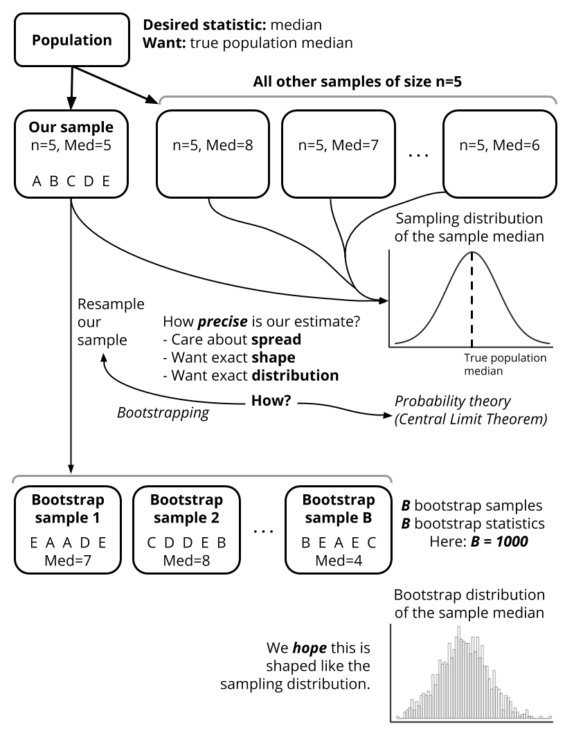
We have looked at one way to estimate the spread of the sampling distribution: bootstrapping! In bootstrapping, we pretend that our sample is the population and look at lots of different samples from this “fake population”. In bootstrapping, we have essentially tried to replicate the idea of getting “all possible samples of a given size from the population”.
6.7.2 The Central Limit Theorem
Another powerful way to understand what the sampling distribution looks like is called the Central Limit Theorem. This is a famous theorem in Statistics that can be stated as follows.
Central Limit Theorem (CLT): Let \(X_1, X_2, \ldots, X_n\) be random variables that denote some value measured on each of \(n\) units in a random sample. Let \(\bar{X}_n = n^{-1}\sum_{i=1}^n X_i\) denote the sample mean of those values. Let all of the random variables \(X_1, \ldots, X_n\) have the same expected value \(\mu\) and variance \(\sigma^2\). Then as the sample size \(n\) get bigger and bigger (grows to infinity), the sample mean \(\bar{X}_n\) becomes normally-distributed with mean \(\mu\) (the true expected value) and variance \(\sigma^2/n\).
What does the CLT tell us? It tells us that with a “sufficiently large” sample size, the sample mean is normally-distributed with a particular mean and variance. This tells us exactly what the sampling distribution is! The center and shape of the sampling distribution are given by a named probability model, the Normal distribution! Let’s focus on the implications of these two parameters:
- The mean: The CLT says that for large samples the sample mean is normally distributed with mean \(\mu\). \(\mu\) is the actual expected value of the random variables! This tells us that the sample mean estimates the population mean correctly, on average. For example, let’s say that the \(X\)’s are house prices, and we want to know the true population mean of house prices. The CLT tells us that, on average, the sample mean will be correct! Another way to say this is that the sample estimates are “unbiased”: underestimates are balanced out by overestimates.
- The variance: The CLT says that for large samples the sample mean is normally distributed with variance \(\sigma^2/n\). Equivalently, the standard deviation is \(\sigma/\sqrt{n}\). This tells us the spread of the sampling distribution! Sample estimates are more likely to be “close to” than “far from” the population parameter \(\mu\). We see that the sample size \(n\) plays a key role. The larger the sample size, the smaller the spread. This matches our intuition that larger samples should generate more precise estimates. In practice, we estimate \(\sigma\) and refer to this estimated standard deviation as the standard error.
Where does the CLT come up in practice? When we fit linear regression and logistic regression models, there were columns in the summarized output labeled “Std. Error”. We have neglected to look at these columns…until NOW. With our understanding of the CLT, we can understand where this column comes from. It turns out that we can apply the CLT to see that our estimated regression coefficients (our betas) are normally-distributed. That is, the theory of the CLT allows us to approximate the sampling distributions of regression coefficients. Behind the scenes, R uses that theory to give us the Standard Error column. This column gives us an estimate of the standard deviation of the sampling distribution for that regression coefficient.
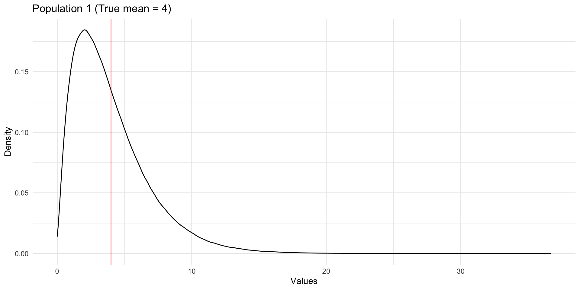
Let’s visualize what is happening with the Central Limit Theorem. Below we have simulated (generated ourselves) data for a full population of cases. The distribution of values in the full population is shown below. The true population mean (expected value) is 4. Beneath, we show the sampling distributions of the sample mean for different sample sizes. We see the CLT in action. The center of the sampling distributions is the expected value 4. The sampling distributions look normally distributed, and the spread decreases with sample size. Note that the original population values do not look normally-distributed, and yet, by the CLT, the sample means are normally-distributed.
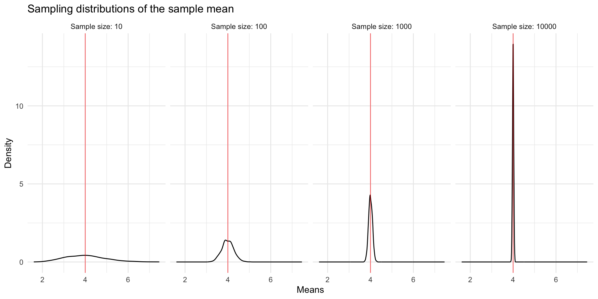
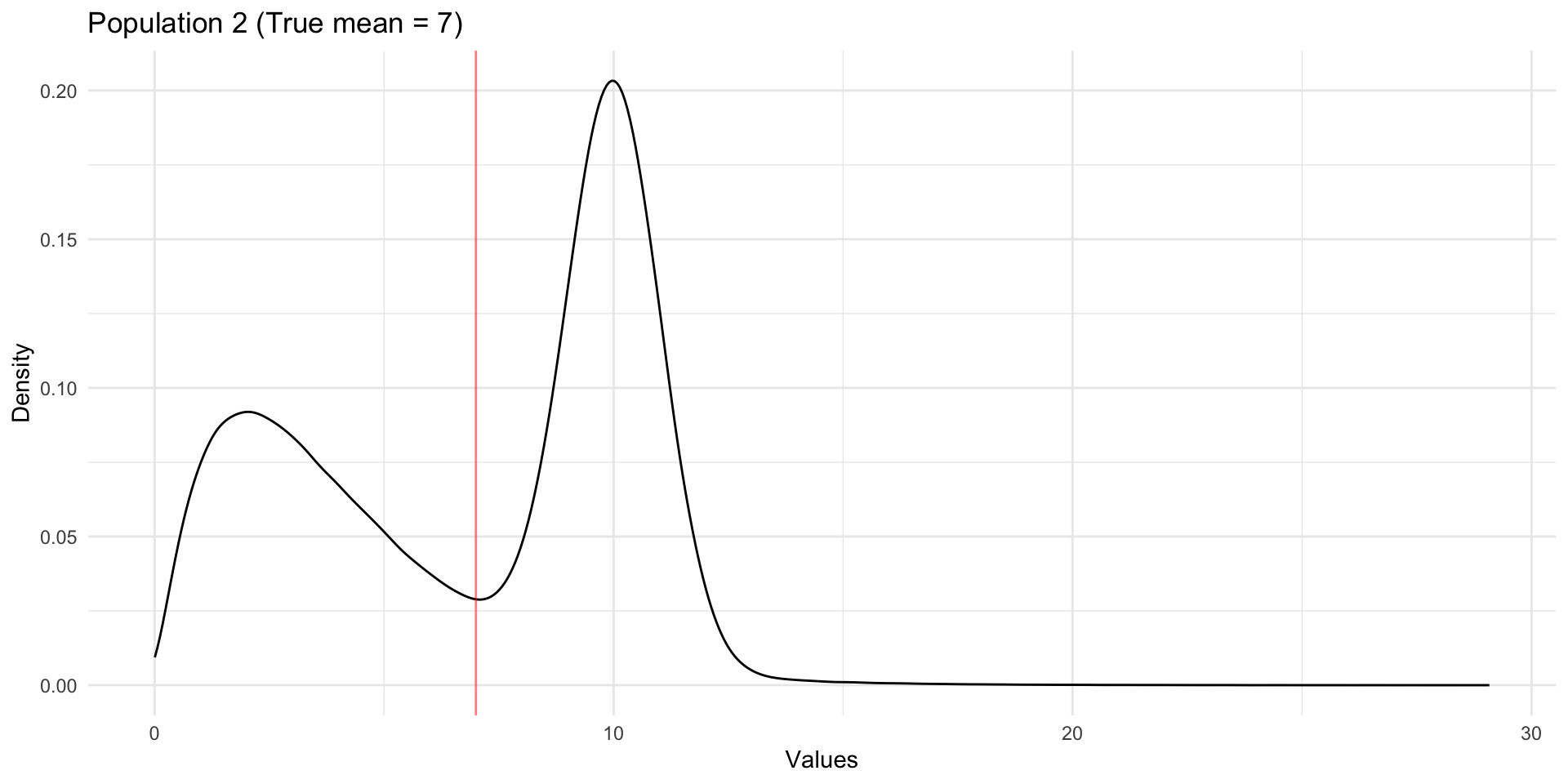
Let’s look at one more example. Again, the population distribution is clearly not normally-distributed, and yet, the sample means are normally-distributed. These normal distributions are centered at the true population mean (expected value) and have smaller and smaller spread with increased sample size.
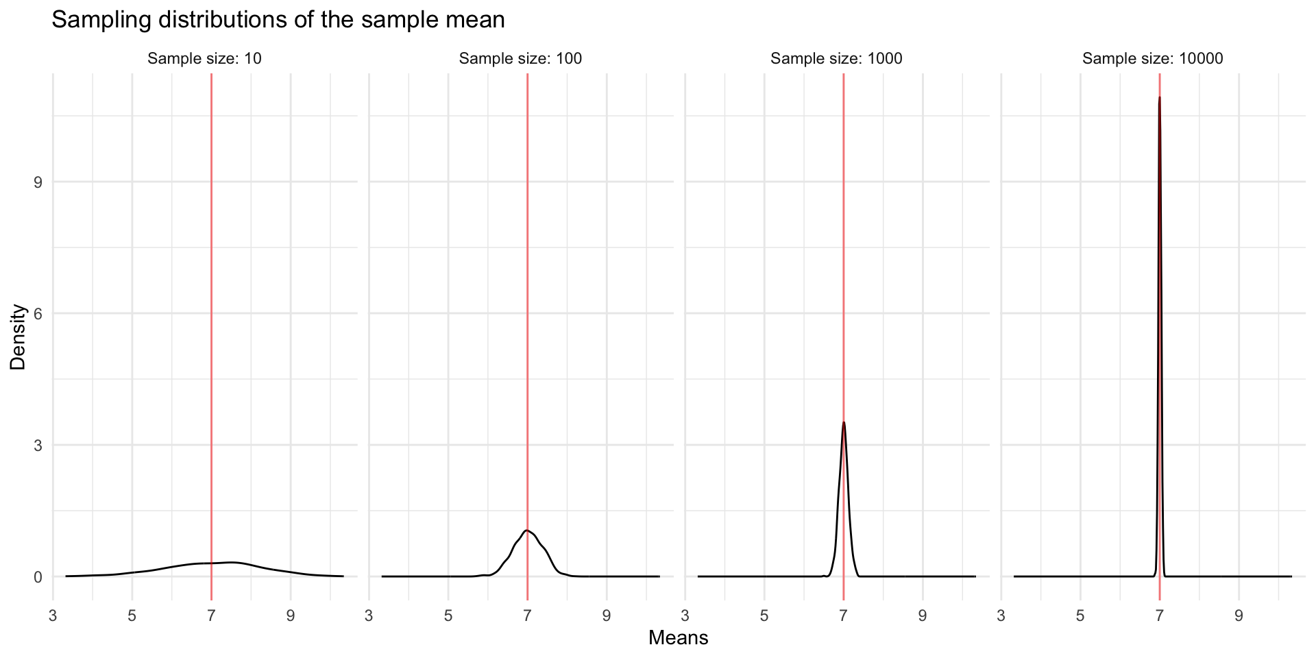
The different ways in which we think about sampling variability in Statistics are shown in the figure below.
