Chapter 6 Randomness and Probability

Now that we have some intuition about random variability, we will formalize some of the concepts of probability and chance.

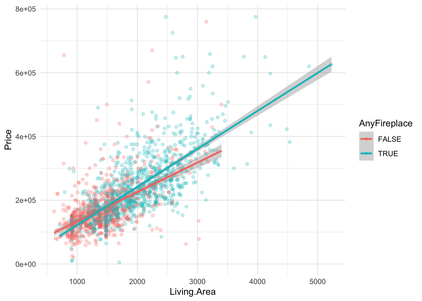
Recall the regression model we built to predict home price as a function of square footage and fireplaces in Section 3.9.

homes <- read.delim("http://sites.williams.edu/rdeveaux/files/2014/09/Saratoga.txt")
homes <- homes %>%
    mutate(AnyFireplace = Fireplaces > 0)
homes %>%
    ggplot(aes(x = Living.Area, y = Price, color = AnyFireplace)) + 
    geom_point(alpha = 0.25) +
    geom_smooth(method = "lm") +
    theme_minimal()

To allow for different slopes among homes with and without a fireplace, we used an interaction term between Living.Area and AnyFireplace. Based on our one sample, we observed a difference in the slopes of $26.85 per square foot.

But is this true for the larger population of homes in the area? Is each square foot worth exactly $26.85 more, on average, in homes with a fireplace than in homes without a fireplace?

lm.home3 <- lm(Price ~ AnyFireplace*Living.Area, data = homes)
tidy(lm.home3)

## # A tibble: 4 × 5
##   term                         estimate std.error statistic  p.value
##   <chr>                           <dbl>     <dbl>     <dbl>    <dbl>
## 1 (Intercept)                   40901.    8235.        4.97 7.47e- 7
## 2 AnyFireplaceTRUE             -37610.   11025.       -3.41 6.61e- 4
## 3 Living.Area                      92.4      5.41     17.1  1.84e-60
## 4 AnyFireplaceTRUE:Living.Area     26.9      6.46      4.16 3.38e- 5

Probably not. In fact, our sample is just one random sample from the larger population of homes in upstate New York at a given time. If we had gotten a slightly different sample of homes, then we would have different estimates for each of the regression coefficients. We explored this sampling variation in Chapter 5 using bootstrapping.

Let’s connect our goals to the terms statistic, estimate, and parameter.

The interaction coefficient is a statistic. It (as well as the other coefficient estimates) is a numerical summary of our data that was estimated from a sample. The actual numerical value of the interaction coefficient in the R output is called the estimate. If we had a census, a full set of data on all homes in upstate New York at a given time, we could fit the same linear regression model. The coefficient estimates given to us by R would represent finite (i.e., at a fixed time) population parameters because they are computed from the whole population at that fixed time, rather than a sample. To conduct statistical inference, we imagine that there is some underlying process governing the populations that we observe at a fixed time, where the parameters of that governing process are what are estimated by our statistical models. By understanding how much statistics vary from sample to sample, we can start to quantify the amount of uncertainty in our estimates. Because the process of obtaining a sample is a type of random process, we will spend some time discussing formal probability.

This chapter briefly discusses the theory of formal probability so that we have terminology and basic concepts to understand and discuss random events. This framework provides a way of thinking about uncertainty, random variability, and average behavior in the long run.

A random process or random event is any process/event whose outcome is governed by chance. It is any process/event that cannot be known with certainty. Examples range from the outcome of flipping a coin to the estimated model coefficients from randomly selected samples.

We’ve used the term “chances” up until now. We are now going to use “probability” as an equivalent word for “chance”.

For a much more in-depth discussion of probability (calculus-based), take STAT/MATH 354 (Probability). For a more detailed understanding of finite populations, underlying governing processes (“superpopulations”), censuses, and general philosophy regarding sampling, take a course on survey statistics.