5.2 Randomization Variability

Another source of random variation in a statistic that can arise is that of random treatment/control group assignments in an experiment. If we could repeat the randomization process in an experiment, each treatment group would be slightly different. The individual composition of the units in the treatment and control groups would differ every time. Sometimes we would randomly over-represent one group of people in the treatment group, and another time we would randomly over-represent another group of people in the treatment group, just by chance. The statistic that we calculate and compare between groups (e.g. a difference in means, a difference in medians, a regression coefficient) would change for every reshuffling of the individuals.

This is another type of random variability. The group composition can vary, and therefore, the statistics that we calculate vary between different randomization.

The important thing to keep in mind is that we only get to see one sample, one particular composition of individuals. But we need to put this one observed sample and statistic in the context of the random variability.

5.2.1 Simulating Randomization into Groups

We have been thinking about estimating the differences in mean arrival delays. But we are interested in whether there is actually a true, real difference because we need to decide whether to have this influence our decisions in booking flights. If the difference is 0, then there is no real difference between morning and afternoon flights.

Let’s use a random sample of 500 flights from the population to investigate this question using a difference approach.

flights_samp500 <- flights %>% 
    sample_n(size = 500) 

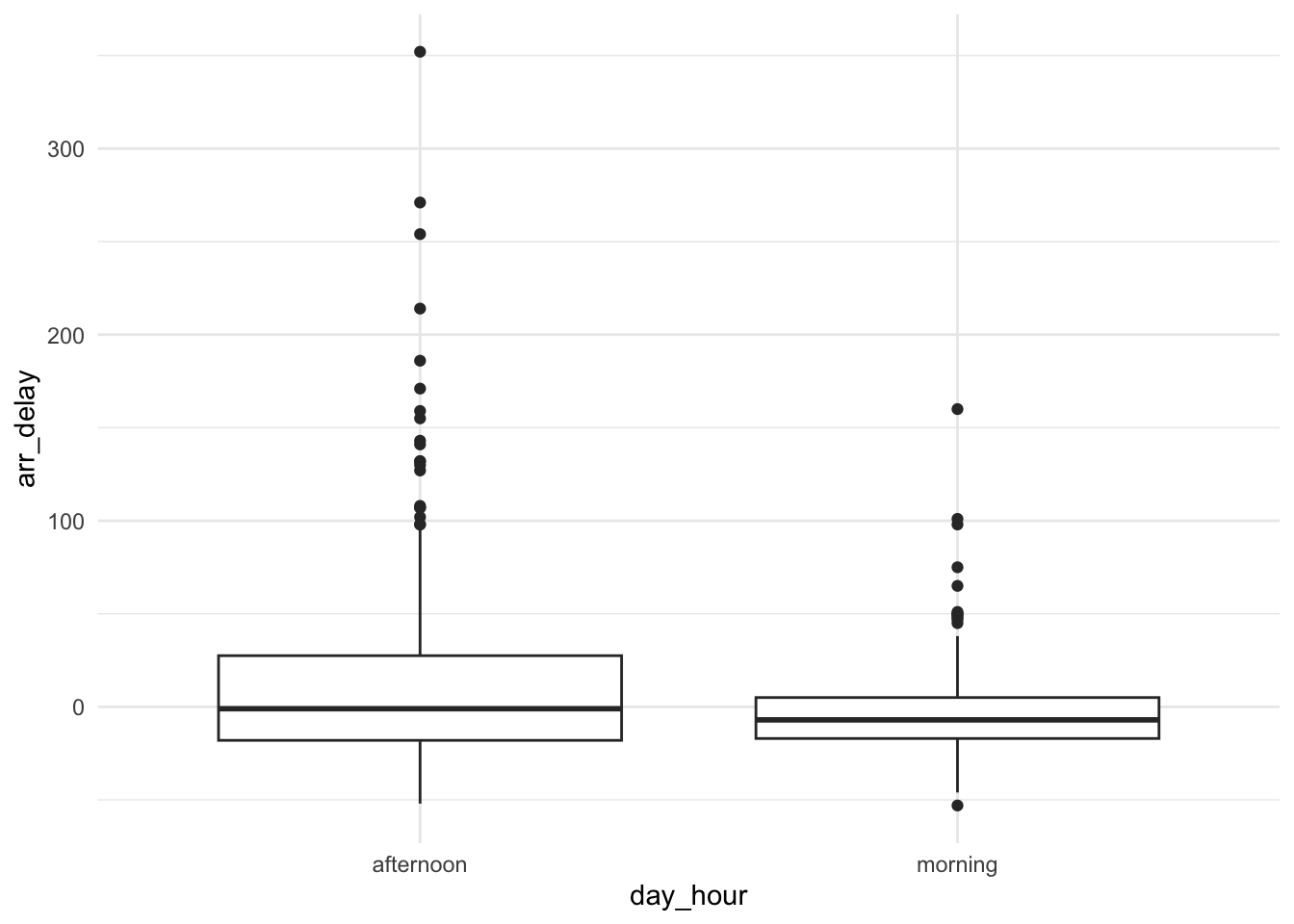
Let’s summarize and visualize the relationship between hour of the day (morning or afternoon) and the arrival delay.

flights_samp500 %>%
    group_by(day_hour) %>%
    summarize(median = median(arr_delay), mean = mean(arr_delay))

## # A tibble: 2 × 3
##   day_hour  median  mean
##   <chr>      <dbl> <dbl>
## 1 afternoon     -1 12.6 
## 2 morning       -7 -2.39

flights_samp500 %>%
    ggplot(aes(x = day_hour, y = arr_delay)) +
    geom_boxplot() +
    theme_minimal()

Based solely on the visual and numerical summaries, are arrival delays less in the morning than in the afternoon?

We don’t know the exact reason why some flights were scheduled in the morning or the afternoon and why one flight might be delayed (it’s probably due to a complex combination of factors). Let’s imagine that a randomization process was used to decide when particular flights were scheduled (morning or afternoon); a flip of a coin to decide morning or afternoon.

We want to compare the mean arrival delays in morning flights and in afternoon flights.

If there were no difference in arrival delays between morning and afternoon flights, then it wouldn’t matter whether a flight left in the morning or afternoon. That is, the day_hour variable would be irrelevant to the arrival delay arr_delay. If that were true, then we could reshuffle the values of day_hour and it wouldn’t change our conclusions.

Wouldn’t it be great if we could see how the mean arrival delays might change if we shuffled the flights between the “morning” group and “afternoon” group, randomly?

In fact, wouldn’t it be great if we could look at every permutation of flights between two groups?

5.2.2 IRL: Randomization Tests

In real life, we don’t often consider every possible permutation (reshuffling of group members) due to the immensely large number of permutations. However, we can randomly reshuffle flights about 1000 times to try to approximate many of those permutations. Such a procedure is called a randomization or permutation procedure. There are three main steps:

1. Hypothesis

Our null hypothesis (a hypothesis that is conservative/not interesting/does not elicit action) is that there is no relationship between time of day and the mean arrival delay.

2. Generate and Calculate

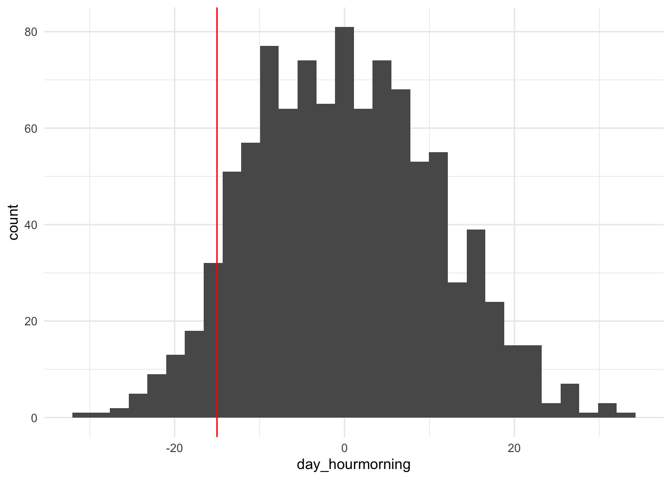
We can generate 1000 new data sets based on randomly reshuffling the labels of day_hour. For each of these data sets, we calculate the difference in mean arrival delay between morning and afternoon groups.

3. Visualize

The histogram below shows the histogram of differences in means if the null hypothesis were true. The vertical line shows the observed difference in means.

Do you think that the mean arrival delay is different for morning and afternoon? Is the observed difference in means likely to have occurred if there were no relationship?

We will return to the ideas of testing hypotheses later in the course.