4.2 Fitting the Model

Based on observed data that includes an indicator variable for the responses (\(Y=1\) for success, \(Y=0\) for failure) and predictor variables, we need to find the slope coefficients, \(\beta_0\),…,\(\beta_k\) that best fits the data. The way we do this is through a technique called maximum likelihood estimation. We will not discuss the details in this class; we’ll save this for an upper level statistics class such as Mathematical Statistics.

In R, we do this with the generalized linear model function, glm().

For a data set, let’s go back in history to January 28, 1986. On this day, the U.S. space shuttle called Challenger took off and tragically exploded about one minute after the launch. After the incident, scientists ruled that the disaster was due to an o-ring seal failure. Let’s look at experimental data on the o-rings prior to the fateful day.

require(vcd)
data(SpaceShuttle)

SpaceShuttle %>%
  filter(!is.na(Fail)) %>%
  ggplot(aes(x = factor(Fail), y = Temperature) )+ 
  geom_boxplot() +
  theme_minimal()

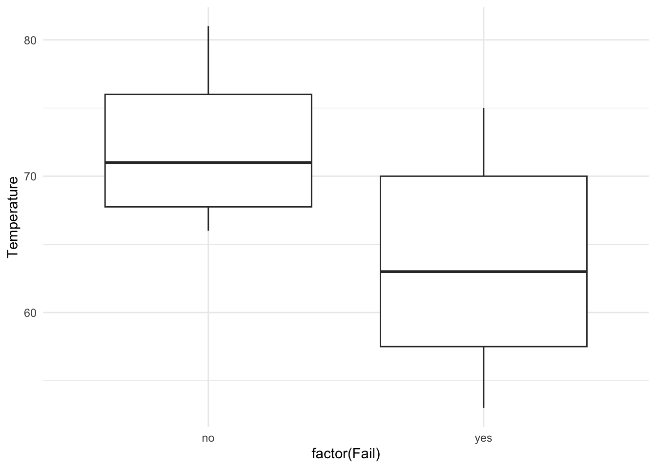
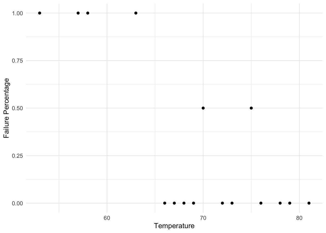
What are the plots above telling us about the relationship between chance of o-ring failure and temperature?

Let’s fit a simple logistic regression model with one explanatory variable to predict the chance of o-ring failure (which is our “success” here – we know it sounds morbid) based on the temperature using the experimental data.

SpaceShuttle <- SpaceShuttle %>%
  mutate(Fail = ifelse(Fail == 'yes', 1, 0))

model.glm <- SpaceShuttle %>%
  with(glm(Fail ~ Temperature, family = binomial))

model.glm %>% 
  tidy()

## # A tibble: 2 × 5
##   term        estimate std.error statistic p.value
##   <chr>          <dbl>     <dbl>     <dbl>   <dbl>
## 1 (Intercept)   15.0       7.38       2.04  0.0415
## 2 Temperature   -0.232     0.108     -2.14  0.0320

Based on a logistic regression model, the predicted log odds of an o-ring failure is given by

\[\log\left(\frac{\hat{p}}{1-\hat{p}}\right) = 15.0429 -0.2322\cdot Temperature\]