Although the term longitudinal naturally suggests that data are collected over time, the models and methods we will discuss broadly apply to any kind of repeated measurement data. That is, although repeated measurements most often take place over time, this is not the only way that measures may be taken repeatedly on the same unit. For example,
The units may be human subjects. For each subject, reduction in diastolic blood pressure is measured on several occasions, each involving the administration of a different dose of anti-hypertensive medication. Thus, the subject is measured repeatedly with varying doses.
The units may be trees in a forest. For each tree, measurements of the tree’s diameter are made at several different points along the tree’s trunk. Thus, the tree is measured repeatedly over positions along the trunk.
The units may be pregnant female rats. Each rat gives birth to a litter of pups, and the birth weight of each pup is recorded. Thus, the rat is measured repeatedly over each of her pups. The third example is slightly different from the other two in that there is no natural order to the repeated measurements.
Thus, the methods will apply more broadly than the strict definition of the term longitudinal data indicates – the term will mean, to us, data in the form of repeated measurements that may well be over time but may also be over some other set of conditions. Because time is most often the measurement condition, however, many of our examples will involve repeated measurement over time. We will use the term outcome to denote the measurement of interest. Because units are often human or animal subjects, we use the terms unit, individual, and subject interchangeably.
6.1 Sources of Variation
We now consider why the values of a characteristic that we might observe vary over time.
Biological variation: It is well-known that biological entities are different. However, living things of the same type tend to be similar in their characteristics; they are not the same (except perhaps in the case of genetically-identical clones). Thus, even if we focus on rats of the same genetic strain, age, and gender, we expect variation in the possible weights of such rats that we might observe due to inherent, natural biological variation. This is variation due to genetics, environmental, and behavioral factors. Thus, this variation is at the unit-level, so we see between unit variation.
Variation due to Condition or Time : Entities change over time and under different conditions. Suppose we consider rats over time or under various dietary conditions. In that case, we expect variation in the possible weights of such rats that we might observe due to variation due to condition or time. Thus, this variation is at the observation-level so we see within unit variation.
Measurement error: We have discussed rat weight as though once we have a rat in hand, we may know its weight exactly. However, a scale must be used. Ideally, a scale should register the true weight of an item each time it is weighed, but because such devices are imperfect, scale measurements on the same item may vary time after time. The amount by which the measurement differs from the truth may be considered an error, i.e., a deviation up or down from the true value that could be observed with a perfect device. A fair or unbiased device does not systematically register high or low most of the time; rather, the errors may go in either direction with no pattern. Thus, this variation is typically at the observation-level, so we see within unit variation.
There are still further sources of variation that we could consider. They could be at the unit-level or the observational-level. For now, the important message is that, in considering statistical models, it is critical to be aware of different sources of variation that cause observations to vary.
With cross-sectional data (one observed point in time in units sampled from across the population - no repeated measures), we
cannot distinguish between the types of variation
use explanatory variables to try and explain any sources of variation (biological and other)
use model error as a catch-all to account for any leftover variation (measurement or other)
With longitudinal data, since we have repeated measurements on units, we
separate variation within units (measurement and others) from variation between units (biological and others)
use time-varying explanatory variables to try and explain within unit variation
use time-invariant explanatory variables to try and explain between unit variation
use probability models to account for left over within or between variation
6.2 Data Examples
We can consider several real datasets from various applications to put things into a firmer perspective. These will not only provide us with concrete examples of longitudinal data situations but also illustrate the range of ways that data may be collected and the types of measurements that may be of interest.
6.2.1 Example 1: The orthodontic study data of Potthoff and Roy (1964).
6.2.1.1 Data Context
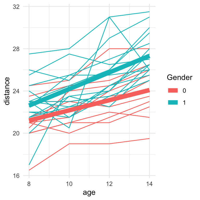
A study was conducted involving 27 children, 16 boys and 11 girls. On each child, the distance (mm) from the center of the pituitary to the pterygomaxillary fissure was made at ages 8, 10, 12, and 14 years of age. In the plot below, the distance measurements are plotted against the age of each child. The trajectory for each child is connected by a solid line so that individual child patterns may be seen, and the color of the lines denotes girls (0) and boys (1).
dat <-read.table("./data/dental.dat", col.names=c("obsno", "id", "age", "distance", "gender"))dat %>%ggplot(aes(x = age, y = distance, col =factor(gender))) +geom_line(aes(group = id)) +geom_smooth(method='lm',se=FALSE,lwd=3) +theme_minimal() +scale_color_discrete('Gender')
`geom_smooth()` using formula = 'y ~ x'
Plots like this are often called spaghetti plots, for obvious reasons! Each set of connected points represented one child and their outcome measurements over time.
6.2.1.2 Research Questions
The objectives of the study were to
Determine whether distances over time are larger for boys than for girls
Determine whether the rate of change (i.e., slope) for distance is similar between boys and girls.
Several features are notable from the spaghetti plot of the data:
Each child appears to have his/her own trajectory of distance as a function of age. For any given child, the trajectory looks roughly like a straight line, with some random fluctuations. But from child to child, the features of the trajectory (e.g., its steepness) vary. Thus, the trajectories are all similar in form but vary in their specific characteristics among children. Also, note any unusual trajectories. In particular, there is one boy whose pattern fluctuates more profoundly than those of the other children and one girl whose distance is much “lower” than the others at all time points.
The overall trend is for the distance measurement to increase with age. The trajectories for some children exhibit strict increases with age. In contrast, others show some intermittent decreases (biologically, is this possible? or just due to measurement error?), but still with an overall increasing trend across the entire six-year period.
The distance trajectories for boys seem, for the most part, to be “higher” than those for girls – most of the boy profiles involve larger distance measurements than those for girls. However, this is not uniformly true: some girls have larger distance measurements than boys at some ages.
Although boys seem to have larger distance measurements, the rate of change of the measurements with increasing age seems similar. More precisely, the slope of the increasing (approximate straight-line) relationship with age seems roughly similar for boys and girls. However, for any individual boy or girl, the rate of change (slope) may be steeper or shallower than the evident “typical” rate of change.
To address the questions of interest, we need a formal way of representing the fact that each child has an individual-specific trajectory.
6.2.2 Example 2: Vitamin E diet supplement and growth of guinea pigs
6.2.2.1 Data Context
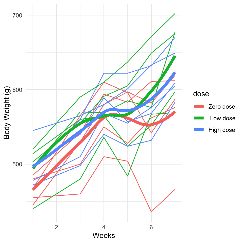
The following data are reported by Crowder and Hand (1990, p. 27). The study concerned the effect of a vitamin E diet supplement on the growth of guinea pigs. 15 guinea pigs were given a growth-inhibiting substance at the beginning of week 1 of the study (time 0, before the first measurement), and body weight was measured at the ends of weeks 1, 3, and 4. At the beginning of week 5, the pigs were randomized into three groups of 5, and vitamin E therapy was started. One group received zero doses of vitamin E, another received a low dose, and the third received a high dose. Each guinea pig’s body weight (g) was measured at the end of weeks 5, 6, and 7. The data for the three dose groups are plotted, in the plot below, with each line representing the body weight of one pig.
dat <-read.table("./data/diet.dat", col.names=c("id", paste("bw.",c(1,3,4,5,6,7),sep=""), "dose" ))dat <- dat %>%gather(Tmp,bw, bw.1:bw.7) %>%separate(Tmp,into=c('Var','time'), remove=TRUE) dat$time <-as.numeric(dat$time)dat$dose <-factor(dat$dose)levels(dat$dose) <-c("Zero dose",' Low dose', 'High dose')dat %>%ggplot(aes(x = time, y = bw, col = dose)) +geom_line(aes( group = id)) +xlab('Weeks') +ylab('Body Weight (g)') +geom_smooth(lwd=2, se=FALSE) +theme_minimal()
`geom_smooth()` using method = 'loess' and formula = 'y ~ x'
6.2.2.2 Research Questions
The primary objective of the study was to
Determine whether the growth patterns differed among the three groups.
As with the dental data, several features of the spaghetti plot are evident:
For the most part, the trajectories for individual guinea pigs seem to increase overall over the study period (although note pig 1 in the zero dose group). Guinea pigs in the same dose group have different trajectories, some of which look like a straight line and others of which seem to have a “dip” at the beginning of week 5, the time at which vitamin E was added in the low and high-dose groups.
The body weight for the zero dose group seems somewhat “lower” than those in the other dose groups.
It is unclear whether the rate of change in body weight on average is similar or different across dose groups. It is unclear that the pattern for individual pigs or “on average” is a straight line, so the rate of change may not be constant. Because vitamin E therapy was not administered until the beginning of week 5, we might expect two “phases” in the growth pattern, before and after vitamin E, making it possibly non-linear.
6.2.3 Example 3: Epileptic seizures and chemotherapy
A common situation is where the measurements are in the form of counts. A response in the form of a count is by nature discrete–counts (usually) take only nonnegative integer values (0, 1, 2, 3,…).
6.2.3.1 Data Context
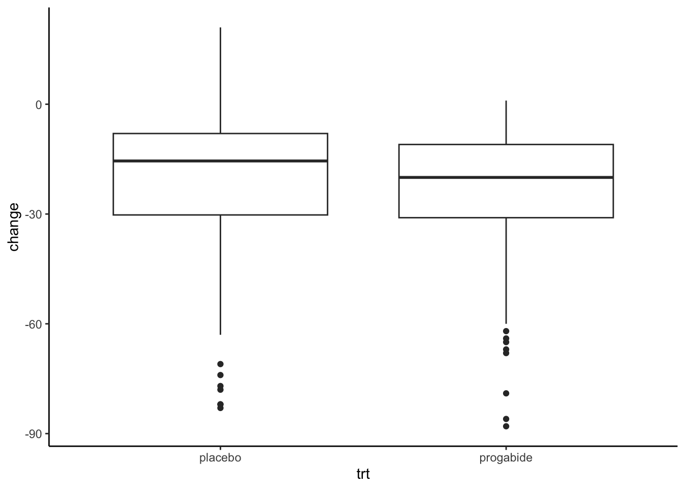
The following data were first reported by Thall and Vail (1990). A clinical trial was conducted in which 59 people with epilepsy suffering from simple or partial seizures were assigned at random to receive either the anti-epileptic drug progabide (subjects 29-59) or an inert substance (a placebo, subjects 1-28) in addition to a standard chemotherapy regimen all were taking. Because each individual might be prone to different rates of experiencing seizures, the investigators first tried to get a sense of this by recording the number of seizures suffered by each subject over the 8 weeks before administering the assigned treatment. It is common in such studies to record such baseline measurements so that the effect of treatment for each subject may be measured relative to how that subject behaved before treatment.
Following the commencement of treatment, each subject’s seizures were counted for four two-week consecutive periods. The age of each subject at the start of the study was also recorded, as it was suspected that the subject’s age might be associated with the effect of the treatment.
The first 10 rows of the long format data for the study are shown below.
Determine whether progabide reduces the rate of seizures in subjects like those in the trial.
Here, we have repeated measurements (counts) on each subject over four consecutive observation periods for each subject. We would like to compare the baseline seizure counts to post-treatment counts, where the latter are observed repeatedly over time following the initiation of treatment. An appropriate analysis would best use this data feature in addressing the main objective. Below is a boxplot of the change from baseline, separated by treatment group (but ignores the repeated measures).
epil %>%mutate(change = y - base) %>%ggplot(aes(x = trt, y = change)) +geom_boxplot() +theme_classic()
Moreover, some counts are quite small; for some subjects, 0 seizures (none) were experienced in some periods. For example, subject 31 in the treatment group experienced only 0, 3, or 4 seizures over the four observation periods. Pretending that the response is continuous would be a lousy approximation of the true nature of the data! Thus, methods suitable for handling continuous data problems like the first three examples would not be appropriate for data like these.
A common approach to handling data in the form of counts is to transform them to some other scale. The motivation is to make them seem more “normally distributed” with constant variance, and the logarithm transformation is used to (hopefully) accomplish this. The desired result is that methods usually used to analyze continuous measurements may be applied.
However, the drawback of this approach is that one is no longer working with the data on the original scale of measurement, the number of seizures in this case. The statistical models the “log number of seizures,” which is not particularly interesting or intuitive. New statistical methods have recently been developed to analyze discrete repeated measurements like counts on the original measurement scale.
6.2.4 Example 4: Maternal smoking and child respiratory health
Another common discrete data situation is where the response is binary; that is, the response may take on only two possible values, which usually correspond to things like
success or failure of a treatment to elicit a desired response
presence or absence of some condition
It would be foolish to even try and pretend such data are approximately continuous!
6.2.4.1 Data Context
The following data come from a very large public health study, the Six Cities Study, undertaken in six small American cities to investigate various public health issues. The full situation is reported in Lipsitz, Laird, and Harrington (1992). The current study focused on the association between maternal smoking and child respiratory health. Each of the 300 children was examined once a year at ages 9–12. The response of interest was “wheezing status, a measure of the child’s respiratory health, which was coded as either”no” (0) or “yes” (1), where “yes” corresponds to respiratory problems. Also recorded at each examination was a code to indicate the mother’s current level of smoking: 0 = none, 1 = moderate, 2 = heavy. The data for the first 5 subjects are summarized below. Missing data are denoted by a “.”.
Smoking at age
Wheezing at age
Subject
City
9
10
11
12
9
10
11
12
1
Portage
2
2
1
1
1
0
0
0
2
Kingston
0
0
0
0
0
0
0
0
3
Portage
1
0
0
.
0
0
0
.
4
Portage
.
1
1
1
.
1
0
0
5
Kingston
1
.
1
2
0
.
0
1
A simplified version of this data is available in R.
Determine how the typical “wheezing” response pattern changes with age
Determine whether there is an association between maternal smoking severity and child respiratory status (as measured by “wheezing”).
It would be pretty pointless to plot the responses as a function of age as we did in the continuous data cases – here, the only responses are 0 or 1! Inspection of subject data suggests something is happening here; for example, subject 5 did not exhibit positive wheezing until his/her mother’s smoking increased in severity.
This highlights that this situation is complex: over time (measured here by the child’s age), an important characteristic, maternal smoking, changes. Contrast this with the previous situations, where the main focus is to compare groups whose membership stays constant over time.
Thus, we have repeated measurements, which are binary to further complicate matters! As with the count data, one might first think about summarizing and transforming the data to allow methods for continuous data to be used; however, this would be inappropriate. As we will see later, methods for dealing with repeated binary responses and scientific questions like those above have been developed.
Another feature of these data is that some measurements are missing for some subjects. Specifically, although the intention was to collect data for each of the four ages, this information is not available for some children and their mothers at some ages; for example, subject 3 has both the mother’s smoking status and wheezing indicator missing at age 12. This pattern would suggest that the mother may have failed to appear with the child for this intended examination.
A final note: In the other examples, units (children, guinea pigs, plots, patients) were assigned to treatments; thus, these may be regarded as controlled experiments, where the investigator has some control over how the factors of interest are “applied” to the units (through randomization). In contrast, in this study, the investigators did not decide which children would have mothers who smoke; instead, they could only observe the smoking behavior of the mothers and the wheezing status of their children. That is, this is an example of an observational study. Because it may be impossible or unethical to randomize subjects to potentially hazardous circumstances, studies of issues in public health and the social sciences are often observational.
As in many observational studies, an additional difficulty is the fact that the thing of interest, in this case, maternal smoking, also changes with the response over time. This leads to complicated issues of interpretation in statistical modeling that are a matter of some debate.
6.3 R: Wide V. Long Format
In R, longitudinal data could be formatted in two ways.
Wide Format: When the observations times are the same for every unit (balanced data), then every unit has a vector of observations of length \(m\), and we can organize the unit’s data into one row per unit, resulting in a data set with \(n\) rows and \(m\) columns that correspond to outcome values (plus other columns that will correspond to an identifier variable and other explanatory variables). See the simulated example below. The first column is an id column to identify the units from each other, the next five columns correspond to the \(m=5\) observations over time, and the next five columns correspond to a time-varying explanatory variable.
n =10m =5(wideD =data.frame(id =1:n, y.1 =rnorm(n), y.2 =rnorm(n), y.3 =rnorm(n), y.4 =rnorm(n), y.5 =rnorm(n),x.1 =rnorm(n), x.2 =rnorm(n), x.3 =rnorm(n), x.4 =rnorm(n), x.5 =rnorm(n))) #Example with 5 repeated observations for 10 units
Long Format: We’ll need the data in long format for most data analysis. We must use a long format when every unit’s observation times differ. Imagine stacking each unit’s observed outcome vectors on top of each other. Similarly, we want to stack the observed vectors of any other explanatory variable we might have on the individuals. In contrast to wide format, it is necessary to have a variable to identify the unit and the observation time.
See below for the R code to convert a data set in wide format to one in long format. Hopefully, the variable names are given in a way that specifies the variable name and the time order of the values, such as y.1,y.2,...y.5,x.1,x.2,...,x.5.
In the tidyr package, pivot_longer() takes the wide data, the columns (cols) you want to make longer, and the names of two variables you want to create. The first (we use Tmp here) is the variable name containing the variable names of the columns you want to gather. The second (called Value) is the variable name that will collect the values from those columns. See below.
Then, we want to separate the Tmp variable into two variables because they contain information about both the characteristic and time. We can use separate() to separate Tmp into Var and Time, it will automatically detect the . as a separator.
# A tibble: 6 × 4
     id Var   Time   Value
  <int> <chr> <chr>  <dbl>
1     1 y     1     -0.927
2     1 y     2     -2.45
3     1 y     3      0.324
4     1 y     4     -1.20
5     1 y     5      1.37
6     1 x     1     -0.134
Lastly, we want to have one variable called x and one variable called y', and we can get that by pivoting the variableVarwider into two columns with the values that come fromValue`.
# A tibble: 6 × 4
     id Time       y      x
  <int> <chr>  <dbl>  <dbl>
1     1 1     -0.927 -0.134
2     1 2     -2.45   1.23
3     1 3      0.324 -0.770
4     1 4     -1.20   0.557
5     1 5      1.37  -0.396
6     2 1      0.585  0.500
6.4 Notation
In order to
elucidate the assumptions made under different models and methods, and
describe the models and methods more easily,
it is convenient to think of all outcomes collected on the same unit over time or another set of conditions together so that complex relationships among them may be summarized.
Consider the random variable,
\[ Y_{ij} = \text{the }j\text{th measurement taken on unit }i,\quad\quad i= 1,...,n, j =1,...,m\]
Consider the dental study data (Example 1) to make this more concrete. Each child was measured 4 times at ages 8, 10, 12, and 14 years. Thus, we let \(j = 1,..., 4\); \(j\) index the measurement order on a child. To summarize the information on when these times occur, we might further define
\[ t_{ij} = \text{ the time at which the }j\text{ measurement on unit i was taken.}\]
Here, for all children (\(i=1,...,27\)), \(t_{i1} = 8, t_{i2} = 10\), and so on for all children in the study. Thus, \(t_{ij} = t_j\) for all \(i=1,...,n\). If we ignore the gender of the children for the moment, the outcomes for the \(i\)th child, where \(i\) ranges from 1 to 27, are \(Y_{i1},..., Y_{i4}\), taken at times \(t_{i1},...,t_{i4}\). We may summarize the measurements for the \(i\)th child even more succinctly: define the (4 × 1) random vector,
The vector elements are random variables representing the outcomes that might be observed for child \(i\) at each time point. For this data set, the data are balanced because the observation times are the same for each unit, and the data are regular because the observation times are equally spaced apart. Most observational data is not balanced and is often irregular. We can generalize our notation to allow for this type of data by changing \(m\) to \(m_i\), which captures the total number of measurements for the \(i\)th unit,
\[ Y_{ij} = \text{the }j\text{th measurement taken on unit }i, \quad\quad i= 1,...,n, j =1,...,m_i\]
The important message is that it is possible to represent the outcomes for the \(i\)th child in a very streamlined and convenient way. Each child \(i\) has its outcome vector, \(\mathbf{Y}_i\). It often makes sense to think of the data not just as individual outcomes \(Y_{ij}\), some from one child, some from another according to the indices, but rather as vectors corresponding to children, the units–each unit has associated with it an entire outcome vector.
We can also consider explanatory variables. If we have \(p\) explanatory variables, we’ll let the value for the 1st variable, for the ith unit at the jth time, be represented as \(x_{ij1}\). That means that for the ith unit, we can collect all of their values of explanatory variables (across time) in a matrix,
These explanatory variables might be time-invariant such that we have a variable like the treatment group. Alternatively, we might have explanatory variables that are time-varying, such as age in the values observed at each time point may change.
6.4.1 Multivariate Normal Probability Model
We first discussed this in Chapter 2, so feel free to return to [Random Vectors and Matrices].
When we represent the outcomes for the \(i\)th unit as a random vector, \(\mathbf{Y}_i\), it is useful to consider a multivariate model such as the multivariate normal probability model.
The joint probability distribution that is the extension of the univariate version to a (\(m \times 1\)) random vector \(\mathbf{Y}\), each of whose components is normally distributed, is given by \[ f(\mathbf{y}) = \frac{1}{(2\pi)^{m/2}}|\Sigma|^{-1/2}\exp\{ -(\mathbf{y} - \mu)^T\Sigma^{-1}(\mathbf{y} - \mu)/2\}\]
This probability density function describes the probabilities with which the random vector \(\mathbf{Y}\) takes on values jointly in its \(m\) elements.
The form is determined by the mean vector \(\mu\) and covariance matrix \(\Sigma\).
The form of \(f(\mathbf{y})\) depends critically on the term \[(\mathbf{y} -{\mu})^T\Sigma^{-1} (\mathbf{y} -{\mu})\]
The quadratic form of the term pops up in many common methods. You’ll see it in generalized least squares (GLS) and the Mahalanobis distance as a standardized sum of squares. Read the next section if you’d like to think more deeply about this quadratic form.
6.4.1.1 Quadratic Form (Optional)
The pdf of the multivariate normal pdf depends critically on the term \[(\mathbf{y} -{\mu})^T\Sigma^{-1} (\mathbf{y} -{\mu})\]
This is a quadratic form (in linear algebra), so it is a scalar function of the elements of \((\mathbf{y} -\mu)\) and \(\Sigma^{-1}\).
If we refer to the elements of \(\Sigma^{-1}\) as \(\sigma^{jk}\), i.e. \[\Sigma^{-1}=\left(\begin{array}{ccc} \sigma^{11}&\cdots&\sigma^{1m}\\ \vdots&\ddots&\vdots\\ \sigma^{m1}&\cdots&\sigma^{mm}\end{array} \right)\] then we may write \[(\mathbf{y} -{\mu})^T\Sigma^{-1} (\mathbf{y} -{\mu}) = \sum^m_{j=1}\sum^m_{k=1}\sigma^{jk}(y_j-\mu_j)(y_k-\mu_k).\]
Of course, the elements \(\sigma^{jk}\) will be complicated functions of the elements \(\sigma^2_j\), \(\sigma_{jk}\) of \(\Sigma\), i.e. the variances of the \(Y_j\) and the covariances among them.
This term thus depends on not only the squared deviations\((y_j - \mu_j)^2\) for each element in \(\mathbf{y}\) (which arise in the double sum when \(j = k\)), but also on the crossproducts \((y_j - \mu_j)(y_k - \mu_k)\). Each contribution of these squares and cross products is standardized by values \(\sigma^{jk}\) that involve the variances and covariances.
Thus, although it is quite complicated, one gets the suspicion that the quadratic form has an interpretation, albeit more complex, as a distance measure, just as in the univariate case.
To better understand the multivariate distribution, it is instructive to consider the special case \(m = 2\), the simplest example of a multivariate normal distribution (hence the name bivariate).
We also have that the correlation between \(Y_1\) and \(Y_2\) is given by \[\rho_{12} = \frac{\sigma_{12}}{\sigma_1\sigma_2}.\]
Using these results, it is an algebraic exercise to show that (try it!) \[ (\mathbf{y} - \mu)^T\Sigma^{-1}(\mathbf{y} - \mu) = \frac{1}{1-\rho^2_{12}}\left\{ \frac{(y_1-\mu_1)^2}{\sigma^2_1}+\frac{(y_2-\mu_2)^2}{\sigma^2_2}-2\rho_{12}\frac{(y_1-\mu_1)}{\sigma_1}\frac{(y_2-\mu_2)}{\sigma_2}\right\}\]
One component is the sum of squared standardized values (z-scores) \[ \frac{(y_1-\mu_1)^2}{\sigma^2_1}+\frac{(y_2-\mu_2)^2}{\sigma^2_2}\]
This sum is similar to the sum of squared deviations in least squares, with the difference that each deviation is now weighted by its variance. This makes sense–because the variances of \(Y_1\) and \(Y_2\) differ, information on the population of \(Y_1\) values is of a different quality than that on the population of \(Y_2\) values. If the variance is large, the quality of information is poorer; thus, the larger the variance, the smaller the weight, so that information of higher quality receives more weight in the overall measure. Indeed, this is like a distance measure, where each contribution receives an appropriate weight.
In addition, there is an extra term that makes it have a different form than just a sum of weighted squared deviations: \[-2\rho_{12}\frac{(y_1-\mu_1)}{\sigma_1}\frac{(y_2-\mu_2)}{\sigma_2}\]
This term depends on the cross-product, where each deviation is again weighted by its variance. This term modifies the distance measure in a way connected with the association between \(Y_1\) and \(Y_2\) through their cross-product and correlation \(\rho_{12}\). Note that the larger this correlation in magnitude (either positive or negative), the more we modify the usual sum of squared deviations.
Note that the entire quadratic form also involves the multiplicative factor \(1/(1 -\rho^2_{12})\), which is greater than 1 if \(|\rho_{12}| > 0\). This factor scales the overall distance measure by the magnitude of the association.
6.5 Failure of Standard Estimation Methods
6.5.1 Ordinary Least Squares
Imagine we have \(n\) units/subjects, and each unit has \(m\) observations over time. Conditional on \(p\) explanatory variables, we typically assume a linear model for the relationship between the explanatory variables and the outcome,
If we are using ordinary least squares to estimate the slope parameters, we assume the errors represent independent measurement error, \(\epsilon_{ij} \stackrel{iid}{\sim} \mathcal{N}(0,\sigma^2)\).
This can be written using vector and matrix notation with each unit having its outcome vector, \(\mathbf{Y}_i\),
\[\mathbf{Y}_i = \mathbf{X}_i\boldsymbol{\beta} + \boldsymbol\epsilon_i\text{ for each unit } i\] where \(\boldsymbol\epsilon_i \sim \mathcal{N}(0,\sigma^2I)\) and \(\mathbf{X}_i\) is the observations for the explanatory variables for subject \(i\) with \(m\) rows and \(p+1\) columns (a column of 1’s for the intercept plus \(p\) columns that correspond to the \(p\) variables).
If we stack all of our outcome vectors \(\mathbf{Y}\) (and covariate matrices \(\mathbf{X}\)) on top of each other (think Long Format in R),
where \(\boldsymbol{\epsilon} \sim \mathcal{N}(0,\sigma^2I)\) so we are assuming that our errors and thus our data are independent within and between each unit and have constant variance.
6.5.1.1 Estimation
To find the ordinary Least Squares (OLS) estimate \(\widehat{\boldsymbol{\beta}}_{OLS}\), we need to minimize the sum of squared residuals, which can be written with vector and matrix notation,
using \(Cov(\mathbf{A}\mathbf{Y}) = \mathbf{A}Cov(\mathbf{Y})\mathbf{A}^T\), which you can verify.
The OLS estimates of our coefficients are fairly good (unbiased), but the OLS standard errors are wrong unless our data are independent. Since we have correlated repeated measures, we don’t have as much “information” as if they were independent observations.
6.5.2 Generalized Least Squares
If you relax the assumption of constant variance, then the covariance matrix of \(\boldsymbol\epsilon_i\) and thus \(\mathbf{Y}_i\) is
For longitudinal data, this would allow the variability to change over time.
If you relax both the assumptions of constant variance and independence, then the covariance matrix of \(\boldsymbol\epsilon_i\) and thus \(\mathbf{Y}_i\) is
For longitudinal data, this would allow the variability to change over time, and you can account for dependence between repeated measures.
If we assume individual units are independent of each other (which is typically a fair assumption), the covariance matrix for the entire vector of outcomes (for all units and their observations over time) is written as a block diagonal matrix,
If \(\boldsymbol{\Sigma}\) is known, taking the derivative with respect to \(\beta_0,\beta_1,...,\beta_p\), we get a set of simultaneous equations expressed in matrix notation as
An alternative approach is to consider transforming our \(\mathbf{Y}\) and \(\mathbf{X}\) by pre-multiplying by the inverse of the lower triangular matrix from the Cholesky Decomposition of the covariance matrix \(\boldsymbol{\Sigma}\) (\(\mathbf{L}\)), and then find the OLS estimator.
We start by transforming our data so that \(\mathbf{Y}^* = \mathbf{L}^{-1}\mathbf{Y}\), \(\mathbf{X}^*\mathbf{L}^{-1}\mathbf{X}\), and \(\boldsymbol\epsilon^* = \mathbf{L}^{-1}\boldsymbol\epsilon\).
We can rewrite the model as,
\[\mathbf{L}^{-1}\mathbf{Y} = \mathbf{L}^{-1}\mathbf{X}\boldsymbol{\beta} + \mathbf{L}^{-1}\boldsymbol\epsilon\]\[\implies \mathbf{Y}^* = \mathbf{X}^*\boldsymbol{\beta} + \boldsymbol\epsilon^*\] Then, using OLS on these transformed vectors, we get the generalized least squares estimator,
The solution to this problem is to iterate. Estimate \(\boldsymbol{\beta}\) and use that to estimate \(\boldsymbol{\Sigma}\). Repeat.
Other Issues:
If the longitudinal data is balanced, there are \(m(m+1)/2\) parameters in \(\boldsymbol\Sigma_i\) to estimate. That is a lot of parameters (!)
If the longitudinal data is unbalanced, there is no common \(\boldsymbol{\Sigma}_i\) for every unit
The solution to these problems involves simplifying assumptions such as
assuming the errors are independent (not a great solution)
assuming the errors have constant variance (maybe not too bad, depending on the data)
assuming there is some restriction/structure on the covariance function (best option)
We approximate the covariance matrix to get better estimates of \(\boldsymbol\beta\).
If we know the correlation structure of our data, we could use generalized least squares to get better (better than OLS) estimates of our coefficients, and the estimated standard errors would be more accurate.
The two main methods for longitudinal data that we’ll learn are similar to generalized least squares in flavor.
However, we need models that are not only applicable to continuous outcomes but also binary or count outcomes. Let’s first learn about the standard cross-sectional approaches to allow for binary and count outcomes (generalized linear models). Then, we’ll be able to talk about marginal models and mixed effects models.
6.6 Generalized Linear Models
When you have outcome data that is not continuous, we can’t use a least squares approach as it is only appropriate for continuous outcomes. However, we can generalize the idea of a linear model to allow for binary or count outcomes. This is called a generalized linear model (GLM). GLM’s extend regression to situations beyond the continuous outcomes with Normal errors (Nelder and Wedderburn 1972), and they are, in fact, a broad class of models for outcomes that are continuous, discrete, binary, etc.
GLM’s requires a three-part specification:
Distributional assumption for \(Y\)
Systematic component with \(\mathbf{X}\)
Link function to relate \(E(Y)\) with systematic component
6.6.1 Distributional Assumption
The first assumption you need to make to fit a GLM is to assume a distribution for the outcome \(Y\).
Many distributions you have learned in probability (normal, Bernoulli, binomial, Poisson) belong to the exponential family of distributions that share a general form and statistical properties. GLM’s are limited to this family of distributions.
One important statistical property of the exponential family is that the variance can be written as a scaled function of the mean,
\[Var(Y) = \phi v(\mu)\quad \text{ where } E(Y) = \mu\]
where \(\phi>0\) is a dispersion or scale parameter and \(v(\mu)\) is a variance function of the mean.
6.6.2 Systematic Component
For a GLM, the mean or a transformed mean can be expressed as a linear combination of explanatory variables, which we’ll notate as \(\eta\):
You’ll need to decide which explanatory variables should be used to model the mean. This may include a time variable (e.g., age, time since baseline, etc.) and other unit characteristics that are time-varying or time-invariant. We’ll refer to this as the mean model.
6.6.3 Link Function
Lastly, the chosen link function transforms the mean and links the explanatory variables to that transformed mean.
This link function, \(g()\), allows us to use a linear function to model positive counts and binary variables.
There are canonical link functions for each distribution in the exponential family.
Normal (linear regression)
\(v(\mu) = 1\)
\(g(\mu) = \mu\) (identity)
Bernoulli/Binomial (m=1) (logistic regression)
\(v(\mu)=\mu(1-\mu)\)
\(g(\mu) = \log(\mu/(1-\mu))\) (logit)
Binomial
\(v(\mu)=m\mu(1-\mu)\)
\(g(\mu) = \log(\mu/(1-\mu))\) (logit)
Poisson (poisson regression)
\(v(\mu)=\mu\)
\(g(\mu) = \log(\mu)\) (log)
For the Six City Study, we can fit a model to predict whether or not a child has respiratory issues as a function of age and maternal smoking, ignoring the repeated measures on each child with the following R code. Notice we need to specify the mean model using the formula notation resp ~ age + smoke, the family of the distribution we assume for our outcome family = binomial and the link function `link = ’logit” we use to connect the linear model to the mean. With this set of assumptions, we are fitting a logistic regression model.
summary(glm(resp ~ age + smoke, data = ohio, family =binomial(link ='logit')))
Call:
glm(formula = resp ~ age + smoke, family = binomial(link = "logit"),
    data = ohio)

Coefficients:
            Estimate Std. Error z value Pr(>|z|)
(Intercept) -1.88373    0.08384 -22.467   <2e-16 ***
age         -0.11341    0.05408  -2.097   0.0360 *
smoke        0.27214    0.12347   2.204   0.0275 *
---
Signif. codes:  0 '***' 0.001 '**' 0.01 '*' 0.05 '.' 0.1 ' ' 1

(Dispersion parameter for binomial family taken to be 1)

    Null deviance: 1829.1  on 2147  degrees of freedom
Residual deviance: 1819.9  on 2145  degrees of freedom
AIC: 1825.9

Number of Fisher Scoring iterations: 4
A marginal model for longitudinal data has a four-part specification, and the first three parts are similar to a GLM.
6.7.1 Model Specification
A distributional assumption about \(Y_{ij}\). We assume a distribution from the exponential family. We will only use this assumption to determine the mean and variance relationship.
A systematic component which is the mean model, \(\eta_{ij} = \mathbf{x}_{ij}^T\boldsymbol\beta\), which get connected to the mean through
a link function: The conditional expectation \(E(Y_{ij}|x_{ij}) = \mu_{ij}\) is assumed to depend on explanatory variables through a given link function (similar to GLM),
Note: This implies that given \(\mathbf{x}_{ij}\), there is no dependence of \(Y_{ij}\) on \(\mathbf{x}_{ik}\) for \(j\not=k\) (warning: this might not hold if \(Y_{ij}\) predicts \(\mathbf{x}_{ij+1}\)).
The conditional variance of each \(Y_{ij}\), given explanatory variables, depends on the mean according to
Note: The \(\phi\) (phi parameter) is a dispersion parameter and scales variance up or down.
Covariance Structure: The conditional within-subject association among repeated measures is assumed to be a function of a set of association parameters \(\boldsymbol\alpha\) (and the means \(\mu_{ij}\)). We choose a working correlation structure for \(Cor(\mathbf{Y}_i)\) from our familiar structures: Compound Symmetry/Exchangeable, Exponential/AR1, Gaussian, Spherical, etc. See [Autocorrelation Function] in Chapter 3 for examples.
Note: We may use the word “association” rather than correlation so that it applies in cases where the outcome is not continuous.
Based on the model specification, the covariance matrix for \(\mathbf{Y}_i\) is
where \(\mathbf{A}_i\) is a diagonal matrix with \(Var(Y_{ij}|X_{ij}) = \phi v(\mu_{ij})\) along the diagonal. We use the term working correlation structure to acknowledge our uncertainty about the assumed model for the within-subject associations.
6.7.2 Interpretation
We typically discuss the mean associated with a 1 unit increase in an explanatory variable, keeping all other variables constant.
In a marginal model, we explicitly model the overall or marginal mean, \(E(Y_{ij}|X_{ij})\).
For a continuous outcome (with identity link function), the expected response of \(Y_{ij}\) for the value of \(X_{ij} = x\) is
\[E(Y_{ij}|X_{ij}=x) = \beta_0 +\beta_1x \]
The expected response of \(Y_{ij}\) for value of \(X_{ij} = x+1\) is
\[E(Y_{ij}|X_{ij}=x+1) = \beta_0 +\beta_1(x+1) \]
The difference is \[E(Y_{ij}| X_{ij}=x+1) -E(Y_{ij}|, X_{ij}=x)\]\[= \beta_0 +\beta_1(x+1) - (\beta_0 +\beta_1x) = \beta_1 \]
Therefore, in the context of a marginal model, \(\beta_1\) has the interpretation of a difference in population mean.
A 1-unit increase in \(X\) is associated with a \(\beta_1\) difference in the overall mean response, keeping all other variables constant.
6.7.3 Estimation
To estimate the parameters, we will use generalized estimating equations (GEE).
With a continuous outcome, this leads to minimizing the following objective function (a standardized sum of squared residuals),
treating \(\mathbf{V}_i\) as known and where \(\boldsymbol\mu_i\) is a vector of means with elements \(\mu_{ij} = g^{-1}(\mathbf{x}_{ij}^T\boldsymbol\beta)\).
Using calculus, it can be shown that if a minimum exists, it must solve the following generalized estimating equations,
where \(\mathbf{D}_i = \partial\boldsymbol\mu_i/\partial\boldsymbol\beta\) is the gradient matrix.
Depending on the link function, there may or may not be a closed-form solution. If not, the solution requires an iterative algorithm.
Because GEE depends on both \(\boldsymbol\beta\), \(\boldsymbol\alpha\) (parameters for the working correlation matrix) and \(\phi\) (variance scalar), the following iterative two-stage estimation procedure is required:
Step 1. Given current estimates of \(\boldsymbol\alpha\) and \(\phi\), \(V_i\) is estimated, and an updated estimate of \(\boldsymbol\beta\) is obtained as the solution to the generalized estimating equations.
Step 2. Given the current estimate of \(\beta\), updated estimates of \(\boldsymbol\alpha\) and \(\phi\) are obtained from the standardized residuals
Step 3. We iterate between Steps 1 and 2 until convergence has been achieved (estimates for \(\boldsymbol\beta\), \(\boldsymbol\alpha\), and \(\phi\) don’t change).
Starting or initial estimates of \(\boldsymbol\beta\) can be obtained assuming independence.
Note: In estimating the model, we only use our assumption about the mean model,
where \(\mathbf{A}_i\) is a diagonal matrix with \(Var(Y_{ij}|X_{ij}) = \phi v(\mu_{ij})\) along the diagonal.
6.7.3.1 R: Three GEE R Packages
There are three packages to do this in R, gee, geepack, and geeM.
We will use geeM when we have large data sets because it is optimized for large data. The geepack package is nice as it has an anova method to help compare models. The gee package has some nice output.
The syntax for the function geem() in geeM package is
formula: Symbolic description of the model to be fitted
id: Vector that identifies the clusters
data: Optional dataframe
family: Description of the error distribution and link function
constr: A character string specifying the correlation structure. Allowed structures are: “independence”, “exchangeable” (equal correlation), “ar1” (exponential decay), “m-dependent” (m-diagonal), “unstructured”, “fixed”, and “userdefined”.
Mv: for “m-dependent”, the value for m.
require(geeM)
Loading required package: geeM
Loading required package: Matrix
Attaching package: 'Matrix'
The following objects are masked from 'package:tidyr':

    expand, pack, unpack
summary(geem(resp ~ age + smoke, id = id, data = ohio, family =binomial(link ='logit'), corstr ='ar1'))
            Estimates Model SE Robust SE    wald       p
(Intercept)   -1.8980  0.10960   0.11470 -16.550 0.00000
age           -0.1148  0.05586   0.04494  -2.554 0.01066
smoke          0.2438  0.16620   0.17980   1.356 0.17520

 Estimated Correlation Parameter:  0.3992
 Correlation Structure:  ar1
 Est. Scale Parameter:  1.017

 Number of GEE iterations: 3
 Number of Clusters:  537    Maximum Cluster Size:  4
 Number of observations with nonzero weight:  2148
The syntax for the function geeglm() in geepack package is
formula: Symbolic description of the model to be fitted
family: Description of the error distribution and link function
data: Optional dataframe
id: Vector that identifies the clusters
contr: A character string specifying the correlation structure. The following are permitted: “independence”, “exchangeable”, “ar1”, “unstructured” and “userdefined”
zcor: Enter a user defined correlation structure
require(geepack)summary(geeglm(resp ~ age + smoke, id = id, data = ohio, family =binomial(link ='logit'), corstr ='ar1'))
Call:
geeglm(formula = resp ~ age + smoke, family = binomial(link = "logit"),
    data = ohio, id = id, corstr = "ar1")

 Coefficients:
            Estimate  Std.err    Wald Pr(>|W|)
(Intercept) -1.90218  0.11525 272.409   <2e-16 ***
age         -0.11489  0.04539   6.407   0.0114 *
smoke        0.23448  0.18119   1.675   0.1956
---
Signif. codes:  0 '***' 0.001 '**' 0.01 '*' 0.05 '.' 0.1 ' ' 1

Correlation structure = ar1
Estimated Scale Parameters:

            Estimate Std.err
(Intercept)    1.021  0.1232
  Link = identity

Estimated Correlation Parameters:
      Estimate Std.err
alpha    0.491 0.06733
Number of clusters:   537  Maximum cluster size: 4
The syntax for the function gee() in gee package is
gee(formula, id, data, family = gaussian, constr = 'independence',Mv)
formula: Symbolic description of the model to be fitted
family: Description of the error distribution and link function
data: Optional dataframe
id: Vector that identifies the clusters
constr: Working correlation structure: “independence”, “exchangeable”, “AR-M”, “unstructured”
Mv: order of AR correlation (AR1: Mv = 1)
require(gee)
Loading required package: gee
summary(gee(resp ~ age + smoke, id = id, data = ohio, family =binomial(link ='logit'), corstr ='AR-M', Mv =1))
 GEE:  GENERALIZED LINEAR MODELS FOR DEPENDENT DATA
 gee S-function, version 4.13 modified 98/01/27 (1998)

Model:
 Link:                      Logit
 Variance to Mean Relation: Binomial
 Correlation Structure:     AR-M , M = 1

Call:
gee(formula = resp ~ age + smoke, id = id, data = ohio, family = binomial(link = "logit"),
    corstr = "AR-M", Mv = 1)

Summary of Residuals:
    Min      1Q  Median      3Q     Max
-0.1939 -0.1586 -0.1439 -0.1179  0.8821


Coefficients:
            Estimate Naive S.E. Naive z Robust S.E. Robust z
(Intercept)  -1.8982    0.10962 -17.316     0.11468  -16.552
age          -0.1148    0.05586  -2.054     0.04494   -2.554
smoke         0.2438    0.16620   1.467     0.17983    1.356

Estimated Scale Parameter:  1.017
Number of Iterations:  3

Working Correlation
        [,1]   [,2]   [,3]    [,4]
[1,] 1.00000 0.3990 0.1592 0.06352
[2,] 0.39900 1.0000 0.3990 0.15920
[3,] 0.15920 0.3990 1.0000 0.39900
[4,] 0.06352 0.1592 0.3990 1.00000
6.7.3.2 Properties of Estimators
We acknowledge that our working covariance matrix \(\mathbf{V}_i\) only approximates the true underlying covariance matrix for \(\mathbf{Y}_i\), but it is wrong.
Despite incorrectly specifying the correlation structure,
\(\hat{\boldsymbol\beta}\) is consistent (meaning that with high probability \(\hat{\boldsymbol\beta}\) is close to the true \(\boldsymbol\beta\) for very large samples) no matter whether the within-in subject associations are correctly modeled.
In large samples, the sampling distribution of \(\hat{\boldsymbol\beta}\) is multivariate normal with mean \(\boldsymbol\beta\) and the covariance is a sandwich, \(Cov(\hat{\boldsymbol\beta}) = B^{-1}MB^{-1}\) where the bread \(B\) is defined as \[B = \sum^n_{i=1} \mathbf{D}_i^T\mathbf{V}_i^{-1}\mathbf{D}_i\] and the middle (meat or cheese or filling) \(M\) is defined as \[M = \sum^n_{i=1} \mathbf{D}_i^T\mathbf{V}_i^{-1}Cov(\mathbf{Y}_i)\mathbf{V}_i^{-1}\mathbf{D}_i\]
We can plug in estimates of the quantities and get
\[\widehat{Cov}(\hat{\boldsymbol\beta}) = \hat{B}^{-1}\hat{M}\hat{B}^{-1}\] where \[\hat{B} = \sum^n_{i=1} \hat{\mathbf{D}}_i^T\hat{\mathbf{V}}_i^{-1}\hat{\mathbf{D}}_i\] and \[\hat{M} = \sum^n_{i=1} \hat{\mathbf{D}}_i^T\hat{\mathbf{V}}_i^{-1}\widehat{Cov}(Y_i)\hat{\mathbf{V}}_i^{-1}\hat{\mathbf{D}}_i\] and \(\widehat{Cov}(\mathbf{Y}_i) = (\mathbf{Y}_i - \hat{\boldsymbol\mu}_i)(\mathbf{Y}_i-\hat{\boldsymbol\mu}_i)^T\)
This is the empirical or sandwich robust estimator of the standard errors. It is valid even if we are wrong about the correlation structure.
Fun fact: If we happen to choose the right correlation/covariance structure and \(\mathbf{V}_i = \boldsymbol\Sigma_i\), where \(\boldsymbol\Sigma_i = Cov(\mathbf{Y}_i)\), then \(Cov(\hat{\boldsymbol\beta}) = B^{-1}\).
Since we model the conditional expectation \(E(Y_{ij}|\mathbf{x}_{ij}) = \mu_{ij}\) with
\[g(\mu_{ij}) = \mathbf{x}_{ij}^T\beta,\]
we can only make overall population interpretations regarding mean outcome at a given value of \(\mathbf{x}_{ij}\).
We can compare two lists of \(\mathbf{x}\) values, \(\mathbf{x}^*\) and \(\mathbf{x}\) and see how that impacts the population mean via the link function \(g(\mu)\),
The model selection tools we use will be similar to those used in Stat 155. To refresh your memory of how hypothesis testing can be used for model selection, please see my Introduction to Statistical Models Notes.
6.7.4.1 Hypothesis Testing for Coefficients (one at a time)
This section is similar to the t-tests in Stat 155.
To decide which explanatory variables should be in the model, we can test whether \(\beta_k=0\) for some \(k\). If the slope coefficient were equal to zero, the associated variable is essentially not contributing to the model.
In marginal models (GEE), the estimated covariance matrix for \(\hat{\boldsymbol\beta}\) is given by the robust sandwich estimator. The standard error for \(\hat{\beta}_k\) is the square rooted values of the diagonal of this matrix corresponding to \(\hat{\beta}_k\). This is reported in the summary output for Robust SE.
To test the hypothesis \(H_0: \beta_k=0\) vs. \(H_A: \beta_k\not=0\), we can calculate a z-statistic (referred to as a Wald statistic),
\[z = \frac{\hat{\beta}_k}{SE(\hat{\beta}_k)}\]
With GEE, the geem() function provides wald statistics and associated p-values for testing \(H_0: \beta_k= 0\). These p-values come from a Normal distribution because we know that is the asymptotic distribution for these estimators.
geemod <-geem(resp ~ age + smoke, id = id, data = ohio, family =binomial(link ='logit'), corstr ='exchangeable')summary(geemod) #look for Robust SE and wald
            Estimates Model SE Robust SE    wald        p
(Intercept)   -1.8800  0.11480   0.11390 -16.510 0.000000
age           -0.1134  0.04354   0.04386  -2.585 0.009726
smoke          0.2651  0.17700   0.17770   1.491 0.135900

 Estimated Correlation Parameter:  0.3541
 Correlation Structure:  exchangeable
 Est. Scale Parameter:  0.9999

 Number of GEE iterations: 3
 Number of Clusters:  537    Maximum Cluster Size:  4
 Number of observations with nonzero weight:  2148
geemod$beta/sqrt(diag(geemod$var)) #wald statistics by hand
(Intercept)         age       smoke
    -16.510      -2.585       1.491
6.7.4.2 Hypothesis Testing for Coefficients (many at one time)
This section is similar to the nested F-tests in Stat 155.
To test a more involved hypothesis \(H_0: \mathbf{L}\boldsymbol\beta=0\) (to test whether multiple slopes are zero or a linear combo of slopes is zero), we can calculate a Wald statistic (a squared z statistic),
We assume the sampling distribution is approximately \(\chi^2\) with df = # of rows of \(\mathbf{L}\) to calculate p-values (as long as \(n\) is large).
This model selection tool is useful when you have a categorical variable with more than two categories. You may want to check to see if we should exclude the entire variable or whether a particular category has an impact on the model.
With the data example, let’s look at smoking. It is only a binary categorical variable, but let’s run the hypothesis test with the example code from above. So, in this case, we let the matrix \(L\) be equal to a \(1\times 3\) matrix with 0’s everywhere except in the 3rd column so that we’d test: \(H_0: \beta_2 = 0\). Even though we used a different test statistic, we ended up with the same p-value as the approach above.
summary(geemod)
            Estimates Model SE Robust SE    wald        p
(Intercept)   -1.8800  0.11480   0.11390 -16.510 0.000000
age           -0.1134  0.04354   0.04386  -2.585 0.009726
smoke          0.2651  0.17700   0.17770   1.491 0.135900

 Estimated Correlation Parameter:  0.3541
 Correlation Structure:  exchangeable
 Est. Scale Parameter:  0.9999

 Number of GEE iterations: 3
 Number of Clusters:  537    Maximum Cluster Size:  4
 Number of observations with nonzero weight:  2148
b = geemod$betaW = geemod$var(L =matrix(c(0,0,1),nrow=1))
# Hypothesis Testingw2 <-as.numeric( t(L%*%b) %*%solve(L %*% W %*%t(L))%*% (L%*%b)) ## should be approximately chi squared1-pchisq(w2, df =nrow(L)) # p-value
[1] 0.1359
So, the p-value, the probability of getting a test statistic as or more extreme assuming the null hypothesis is true, is around 13%. We do not have enough evidence to reject the null hypothesis. This leads us to believe that smoking could be removed from the model.
Let’s test whether \(H_0: \beta_1 = \beta_2 = 0\), then we let the matrix \(L\) be equal to a \(2\times 3\) matrix with 0’s everywhere except in the 2nd column in row 1 and 3rd column in row 2.
summary(geemod)
            Estimates Model SE Robust SE    wald        p
(Intercept)   -1.8800  0.11480   0.11390 -16.510 0.000000
age           -0.1134  0.04354   0.04386  -2.585 0.009726
smoke          0.2651  0.17700   0.17770   1.491 0.135900

 Estimated Correlation Parameter:  0.3541
 Correlation Structure:  exchangeable
 Est. Scale Parameter:  0.9999

 Number of GEE iterations: 3
 Number of Clusters:  537    Maximum Cluster Size:  4
 Number of observations with nonzero weight:  2148
b = geemod$betaW = geemod$var(L =matrix(c(0,1,0,0,0,1),nrow=2,byrow=TRUE))
# Hypothesis Testingw2 <-as.numeric( t(L%*%b) %*%solve(L %*% W %*%t(L))%*% (L%*%b)) ## should be approximately chi squared1-pchisq(w2, df =nrow(L)) #p-value
[1] 0.01092
We have evidence to suggest that at least one of the variables, age or smoking, has a statistically significant effect on the outcome. As we saw above, we know it must be age, but the model with age and smoking is better than a model with no explanatory variables.
6.7.4.3 Diagnostics
For any linear model with a quantitative outcome and at least one quantitative explanatory variable, we should check to see if the residuals have a pattern.
Ideally, the residual plot should have no obvious pattern, plotting the residuals on the y-axis against a quantitative x-variable. See some example code below.
If there is a pattern, then we are systematically over or under-predicting, and we can use that information to incorporate non-linearity to improve the model.
6.8 Mixed Effects
Let’s return to a continuous outcome setting. Consider the mean response for a specific individual (\(i\)th individual/unit) at a specific observation time (\(j\)th time).
If the mean is constant across observation times (horizontal trend line) and other variables (no X’s), and the same across all individuals, \[\mu_{ij} = \mu\]
If the mean changes linearly across observation times and no other variables impact the mean, and it is the same across all individuals, \[\mu_{ij} = \beta_0 + \beta_1 t_{ij}\]
If the mean increases linearly with an time-varying explanatory variable and it is the same across all individuals, \[\mu_{ij} = \beta_0 + \beta_1 x_{ij}\]
6.8.1 Individual Intercepts
In any situations listed above, individuals may have their own intercept, their own starting level. We can notate that by adding \(b_i\) as an individual deviation from the mean intercept,
\[\mu_{ij} = \mu + b_i\]
\[\mu_{ij} = \beta_0 + b_i + \beta_1 t_{ij}\]
\[\mu_{ij} = \beta_0 + b_i + \beta_1 x_{ij}\]
We could estimate the individual intercepts to find \(b_i\), the difference between the overall mean intercept and an individual’s intercept. If \(b_i = -2\), the individual \(i\) starts -2 units lower in their outcome responses than the average.
6.8.1.1 First Approach: Separate Models
Let’s use the dental data to figure out the overall mean intercept and estimate each deviation from that intercept. The first approach is to fit a separate linear model for each person and look at the intercepts.
However, this stratification approach also allows everyone to have their own slope for age, which we may not want to do. If there is some common growth across persons, we’d like to borrow information across all persons and fit only one model.
6.8.1.2 Second Approach: Fixed Effects Models
To estimate a model with one fixed slope for everyone that allows for individual intercepts, we fit a model often termed a fixed effects model. In this model, we include an indicator variable for every individual id to allow for individual intercepts. This can be quite difficult if we have a large sample size because we are estimating one parameter per person or unit.
An alternative way for individuals to have their own intercept is to assume a probability distribution for the $ b_i$’s such as \(N(0,\sigma_b^2)\) and estimate the variability,\(\sigma^2_b\). This is a random intercept model,
\[Y_{ij} = \beta_0 + b_i + \beta_1x_{ij} + \epsilon_{ij},\quad \quad b_i\stackrel{iid}{\sim} N(0,\sigma^2_b), \epsilon_{ij}\stackrel{iid}{\sim} N(0,\sigma^2_e),\] where \(\epsilon_{ij}\) and \(b_i\) are independent for any \(i\) and \(j\).
library(lme4)summary(lmer(distance ~ age + (1|id), data = dental))
Linear mixed model fit by REML ['lmerMod']
Formula: distance ~ age + (1 | id)
   Data: dental

REML criterion at convergence: 447

Scaled residuals:
   Min     1Q Median     3Q    Max
-3.665 -0.535 -0.013  0.487  3.722

Random effects:
 Groups   Name        Variance Std.Dev.
 id       (Intercept) 4.47     2.11
 Residual             2.05     1.43
Number of obs: 108, groups:  id, 27

Fixed effects:
            Estimate Std. Error t value
(Intercept)  16.7611     0.8024    20.9
age           0.6602     0.0616    10.7

Correlation of Fixed Effects:
    (Intr)
age -0.845
In the output above, you’ll see information about the standardized or scaled residuals.
Below it, you’ll see information on the random effects. In our case, we have a random intercept for each individual that we allowed by adding + (1 | id) to the formula. The 1 indicates intercept, ’ |indicates conditional on, andidrefers to the variable calledid`. We assumed that \(b_i \sim N(0,\sigma^2_b)\) and it has estimated \(\hat{\sigma}^2_b = 4.472\), \(\hat{\sigma}_b = 2.115\). Additionally, we have assumed that our errors are independent with constant variance, \(\hat{\sigma}^2_e = 2.049\), \(\hat{\sigma}_e = 1.432\).
Lastly, we have our fixed effects, the parameters we don’t assume are random, \(\beta_0\) and \(\beta_1\). Those estimates are \(\hat{\beta}_0 = 16.76\) and \(\hat{\beta}_1 = 0.66\).
Now with this random effects model, the addition of a random intercept has induced correlation between observation within an individual because they now share an intercept.
for \(j\not=l\) and this does not depend on \(j\) or \(l\) or \(j-l\). The correlation is constant for any time lags (exchangeable/compound symmetric).
6.8.2 Individual Slopes
Since we have longitudinal data, we can observe each individual’s trajectory over time. Everyone has their own unique growth rate. If that growth rate can be explained with an explanatory variable, we could use an interaction term to allow for that unique growth. Otherwise, we could allow each individual to estimate their own slope.
6.8.2.1 Second Approach: Fixed Effects Models
One could use a fixed effects model and use an interaction term with the id variable to estimate each individual slope, but that is not sustainable for larger data sets.
A more efficient way to allow individuals to have their own slopes is to assume a probability distribution for the slopes (and typically intercepts) by assuming the vector of individual intercept and slope is bivariate Normal with covariance matrix \(G\), \((b_{i0},b_{i1}) \sim N(0,G)\). This is a random slope and intercept model,
\[Y_{ij} = (\beta_0 + b_{i0}) + (\beta_1 + b_{i1})x_{ij} + \epsilon_{ij},\quad \quad (b_{i0},b_{i1}) \sim N(0,G), \epsilon_{ij}\stackrel{iid}{\sim} N(0,\sigma^2_e),\] where \(\epsilon_{ij}\) and \((b_{i0}, b_{i1})\) are independent of each other for any \(i\) and \(j\).
summary(lmer(distance ~ age + (age|id), data = dental))
Linear mixed model fit by REML ['lmerMod']
Formula: distance ~ age + (age | id)
   Data: dental

REML criterion at convergence: 442.6

Scaled residuals:
   Min     1Q Median     3Q    Max
-3.223 -0.494  0.007  0.472  3.916

Random effects:
 Groups   Name        Variance Std.Dev. Corr
 id       (Intercept) 5.4166   2.327
          age         0.0513   0.226    -0.61
 Residual             1.7162   1.310
Number of obs: 108, groups:  id, 27

Fixed effects:
            Estimate Std. Error t value
(Intercept)  16.7611     0.7753   21.62
age           0.6602     0.0713    9.27

Correlation of Fixed Effects:
    (Intr)
age -0.848
In the output above, you’ll see information about the standardized or scaled residuals.
Below it, you’ll see information on the random effects. In our case, we have a random intercept and a random slope for age for each individual that we allowed by adding + (age | id) to the formula. We might read (age | id) as we want to estimate slope | indicates conditional on, and id refers to the variable called id. We assumed that \((b_{i0}, b_{i1}) \sim N(0,G)\). The estimated covariance matrix \(G\) is
Additionally, we have assumed that our errors are independent with constant variance, \(\hat{\sigma}^2_e = 1.72\), \(\hat{\sigma}_e = 1.31\).
Lastly, we have our fixed effects, the parameters we don’t assume are random, \(\beta_0\) and \(\beta_1\). Those estimates are \(\hat{\beta}_0 = 16.76\) and \(\hat{\beta}_1 = 0.66\). You’ll notice that these estimates did not change much at all by adding a random intercept. This will more often happen when modeling a continuous outcome (not when modeling a binary or count outcome).
6.8.3 Multi-level or Hierarchical Model
We can write the random intercept and slope model by creating layers of models. We can write the model for the mean as the level 1 model
\[ = \underbrace{\text{Fixed effects}}_{\text{mean model}} + \underbrace{\text{Random effects}}_{\text{between unit variation}} + \underbrace{text{Error}}_{\text{within unit variation}}\]
where \(\mathbf{X}_i\) is the design matrix for the fixed effects, \(\mathbf{Z}_i\) is the design matrix for the random effects (a subset of columns of \(\mathbf{X}_i\)), \(\boldsymbol\epsilon_i\sim N(0,\boldsymbol\Sigma)\), and \(\mathbf{b}_i\sim N(0,\mathbf{G})\).
The expected response of \(Y_{ij}\) for value of \(X_{ij} = x\) is
\[E(Y_{ij}|X_{ij}=x) = \beta_0 +\beta_1x \]
The expected response of \(Y_{ij}\) for value of \(X_{ij} = x+1\) is
\[E(Y_{ij}|X_{ij}=x+1) = \beta_0 +\beta_1(x+1) \]
The difference is \[E(Y_{ij}| X_{ij}=x+1) -E(Y_{ij}|, X_{ij}=x)\]\[= \beta_0 +\beta_1(x+1) - (\beta_0 +\beta_1x) = \beta_1 \]
Therefore, in the context of a linear mixed effects model, \(\beta_1\) has the interpretation of the subject-specific change as well as the population mean change.
A 1-unit increase in \(X\) is associated with a \(\beta_1\) difference in the subject’s mean response, keeping all other variables constant.
A 1-unit increase in \(X\) is associated with a \(\beta_1\) difference in the overall mean response, keeping all other variables constant.
6.8.7 Estimation
6.8.7.1 Maximum Likelihood Estimation
Mixed Effects Models require specifying the entire distribution. We assume probability models for the random effects and the errors, and thus we could use maximum likelihood estimation to find estimates for our slopes.
If we specify the REML argument in lmer as REML = FALSE, then the lmer function will maximize the log-likelihood function (based on Normal assumptions for the errors and random effects),
where \(\mathbf{V}_i\) is the composite covariance matrix.
Estimates of \(\ beta\)’s are unbiased if the model is correct (random effects and mean model).
All parameter estimates are consistent if the model is correct.
All parameter estimates are asymptotically unbiased; as \(n\rightarrow\infty\), they become unbiased (if model is correct).
Estimates are asymptotically Normal; as \(n\rightarrow\infty\), the sampling distribution becomes more Normal.
Estimates of variance of random effects are biased with finite \(n\).
6.8.7.2 Restricted Maximum Likelihood Estimation
Patterson and Thompson (1971) and Harville (1974) provided technical solutions to the issues of maximum likelihood. They suggested maximizing the likelihood of observing the sample residuals rather than the sample data. This is referred to as restricted maximum likelihood or REML and is implemented in lmer by default when REML = TRUE.
REML Algorithm:
Estimate fixed effects using OLS.
Write down the likelihood of residuals in terms of residuals and variance parameters.
Then maximize likelihood with respect to variance parameters.
Another REML Algorithm:
Split the likelihood into one part about the mean and one part about the variance.
First, maximize the variance part to get estimates of the variance parameters
Then maximize the part about the mean using the estimated variance.
After some complicated mathematics, you ultimately end up maximizing the following with respect the parameters of \(\mathbf{V}_i\)
and \(\hat{\boldsymbol\beta}= (\sum^n_{i=1}\mathbf{X}_i^T\mathbf{V}_i\mathbf{X}_i)^{-1}(\sum^n_{i=1}\mathbf{X}_i^T\mathbf{V}_i\mathbf{Y}_i)\) are the GLS estimates.
Advantages of REML
Less bias in variance estimators.
\(\hat{\boldsymbol\beta}\) is still unbiased as long as the model is correct.
Disadvantages of REML
You can only compare models that differ in their variance components with REML.
You cannot compare models with differing fixed effects because you didn’t maximize the full information (use ML for this).
6.8.8 Model Selection
6.8.8.1 Hypothesis Testing for Fixed Effects (one at a time)
To decide which fixed effects should be in the model, we can test whether \(\beta_k=0\).
The estimated covariance matrix for \(\hat{\boldsymbol\beta}\) is \[\widehat{Cov}(\hat{\boldsymbol\beta}) = \left\{ \sum^n_{i=1} \mathbf{X}_i^T\hat{\mathbf{V}}_i\mathbf{X}_i \right\}^{-1}\]
The standard error for \(\hat{\beta}_k\) is the square rooted values of the diagonal of this matrix corresponding to \(\hat{\beta}_k\). This is what is reported in the summary output.
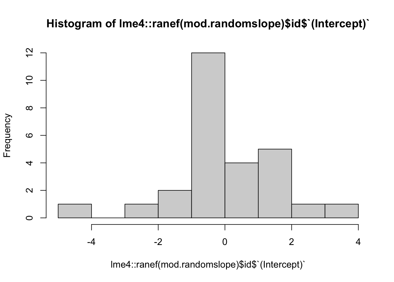
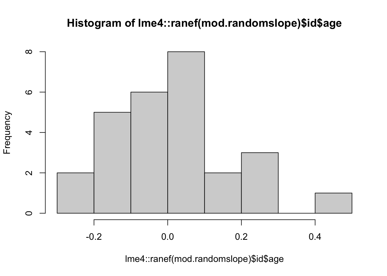
mod.randomslope <-lmer(distance~age + (age|id), data = dental)lme4::fixef(mod.randomslope)
(Intercept)         age
    16.7611      0.6602
vcov(mod.randomslope)
2 x 2 Matrix of class "dpoMatrix"
            (Intercept)       age
(Intercept)     0.60105 -0.046855
age            -0.04685  0.005077
summary(mod.randomslope)
Linear mixed model fit by REML ['lmerMod']
Formula: distance ~ age + (age | id)
   Data: dental

REML criterion at convergence: 442.6

Scaled residuals:
   Min     1Q Median     3Q    Max
-3.223 -0.494  0.007  0.472  3.916

Random effects:
 Groups   Name        Variance Std.Dev. Corr
 id       (Intercept) 5.4166   2.327
          age         0.0513   0.226    -0.61
 Residual             1.7162   1.310
Number of obs: 108, groups:  id, 27

Fixed effects:
            Estimate Std. Error t value
(Intercept)  16.7611     0.7753   21.62
age           0.6602     0.0713    9.27

Correlation of Fixed Effects:
    (Intr)
age -0.848
To test the hypothesis \(H_0: \beta_k=0\) vs. \(H_A: \beta_k\not=0\), we can calculate a z-statistic,
\[z = \frac{\hat{\beta}_k}{SE(\hat{\beta}_k)}\]
There is debate about the appropriate distribution of this statistic, which is why p-values are not reported in the output. However, if you have an estimate that is large relative to the standard error, that indicates that it is significantly different from zero.
To test a more involved hypothesis \(H_0: \mathbf{L}\boldsymbol\beta=0\) (for multiple rows), we can calculate a Wald statistic,
Then we assume the sampling distribution is approximately \(\chi^2\) with df = # of rows of \(\mathbf{L}\) to calculate p-values (as long as \(n\) is large). Below is some example R code.
b =fixef(mod1)W =vcov(mod1)L =matrix(c(0,0,0,1),nrow=1)L%*%b(se =sqrt(diag(L%*%W%*%t(L)))) ##Robust SE's for Lb##95% Confidence Interval (using Asymptotic Normality)L%*%b -1.96*seL%*%b +1.96*se##Hypothesis Testingw2 <-as.numeric( t(L%*%b) %*%solve(L %*% W %*%t(L))%*% (L%*%b)) ## should be approximately chi-squared1-pchisq(w2, df =nrow(L)) #p-value
Let’s consider the data on the guinea pigs. In particular, we fit a model with a random intercept and dose, time, and the interaction between dose and time. If we want to know if the interaction term is necessary, we need to test whether both of their slopes for the interaction term are equal to 0.
w2 <-as.numeric( t(L%*%b) %*%solve(L %*% W %*%t(L))%*% (L%*%b))1-pchisq(w2, df =nrow(L)) #We don't have enough evidence to reject null (thus, don't need interaction term)
[1] 0.1695
Lastly, another option is a likelihood ratio test. Suppose we have two models with the same random effects and covariance models.
Full model: \(M_f\) has \(p\) columns in \(\mathbf{X}_i\) and thus \(p\) fixed effects \(\beta_0,...,\beta_{p-1}\).
Nested model: \(M_n\) has \(k\) columns such that \(k < p\) and \(p-k\) fixed effects \(\beta_l = 0\).
If we use maximum likelihood estimation, it makes sense to compare the likelihood of two models.
\(H_0:\) nested model is true, \(H_A:\) full model is true
If we take the ratio of the likelihoods from the nested model and full model and plug in the maximum likelihood estimators, then we have another statistic.
The sampling distribution of this statistic is approximately chi-squared with degrees of freedom equal to the difference in the number of parameters between the two models.
mod.pigsML <-lmer(bw ~ dose*time + (1|id), data = pigs, REML=FALSE)mod.pigsML2 <-lmer(bw ~ dose+time + (1|id), data = pigs, REML=FALSE)anova(mod.pigsML,mod.pigsML2)
1-pchisq(Dstat,df =2) #df = difference in number of parameters
'log Lik.' 0.1645 (df=6)
6.8.8.2 Information Criteria for Choosing Fixed Effects
To use BIC to choose models, you must use maximum likelihood estimation instead of REML.
mod.pigsML <-lmer(bw ~ dose*time + (1|id), data = pigs, REML=FALSE)summary(mod.pigsML)
Linear mixed model fit by maximum likelihood  ['lmerMod']
Formula: bw ~ dose * time + (1 | id)
   Data: pigs

      AIC       BIC    logLik -2*log(L)  df.resid
    892.9     912.9    -438.4     876.9        82

Scaled residuals:
   Min     1Q Median     3Q    Max
-2.656 -0.405  0.034  0.684  2.167

Random effects:
 Groups   Name        Variance Std.Dev.
 id       (Intercept) 1059     32.5
 Residual              675     26.0
Number of obs: 90, groups:  id, 15

Fixed effects:
                   Estimate Std. Error t value
(Intercept)          469.69      18.52   25.36
dose Low dose          4.84      26.19    0.18
doseHigh dose         11.15      26.19    0.43
time                  16.03       2.40    6.66
dose Low dose:time     6.53       3.40    1.92
doseHigh dose:time     3.60       3.40    1.06

Correlation of Fixed Effects:
            (Intr) dsLwds dsHghd time   dsLds:
doseLowdose -0.707
doseHighdos -0.707  0.500
time        -0.563  0.398  0.398
dosLowds:tm  0.398 -0.563 -0.281 -0.707
dosHghds:tm  0.398 -0.281 -0.563 -0.707  0.500
BIC(mod.pigsML)
[1] 912.9
mod.pigsML2 <-lmer(bw ~ dose+time + (1|id), data = pigs, REML=FALSE)summary(mod.pigsML2)
Linear mixed model fit by maximum likelihood  ['lmerMod']
Formula: bw ~ dose + time + (1 | id)
   Data: pigs

      AIC       BIC    logLik -2*log(L)  df.resid
    892.5     907.5    -440.2     880.5        84

Scaled residuals:
    Min      1Q  Median      3Q     Max
-2.8167 -0.4878 -0.0196  0.6569  2.1617

Random effects:
 Groups   Name        Variance Std.Dev.
 id       (Intercept) 1053     32.5
 Residual              708     26.6
Number of obs: 90, groups:  id, 15

Fixed effects:
              Estimate Std. Error t value
(Intercept)     455.05      16.50   27.58
dose Low dose    33.13      21.65    1.53
doseHigh dose    26.77      21.65    1.24
time             19.40       1.42   13.64

Correlation of Fixed Effects:
            (Intr) dsLwds dsHghd
doseLowdose -0.656
doseHighdos -0.656  0.500
time        -0.374  0.000  0.000
BIC(mod.pigsML2) #This model has a lower BIC
[1] 907.5
6.8.8.3 Hypothesis Testing for Random Effects
The main way to compare models with different random effects is to compare two models with the same fixed effects. Then use a likelihood ratio test with ML to compare the two models’ fit. Again, the null hypothesis is that the smaller model (less complex model – fewer parameters) is the true model. If we see a higher log-likelihood with the more complex model, we may get a small p-value suggesting that we reject the null hypothesis in favor of the more complex model.
Below, I compare two models fit to the guinea pig data. They have the same fixed effects, but I allowed one to have a random slope and intercept while the other only has a random slope. By comparing these two models, we find that the one with a random slope and intercept better fits the data. Thus we reject the null hypothesis that the model with the random intercept is true in favor of the model with the random slope and intercept.
mod.pigsML2 <-lmer(bw ~ dose+time + (1|id), data = pigs, REML=FALSE)mod.pigsML3 <-lmer(bw ~ dose+time + (time|id), data = pigs, REML=FALSE)anova(mod.pigsML2, mod.pigsML3)
which can be rewritten as the weighted average of the population marginal mean, \(\mathbf{X}_i\hat{\boldsymbol\beta}\) and the individual response \(\mathbf{Y}_i\),