As we introduced at the beginning of the course, most models we use for data are written in terms of model components of a deterministic or systematic component plus noise or error,
The deterministic component would generally give the average outcome as a function of \(x_t\), which could represent time/space and/or explanatory variables measured across time/space.
In Stat 155 (Introduction to Statistical Modeling), we model the deterministic component with linear combinations of explanatory variables, \(f(\mathbf{x}) = \beta_0+\beta_1x_1+\beta_2x_2+\cdots+\beta_px_p\), and we assume the noise was independent.
In Stat 253 (Statistical Machine Learning), we learn parametric and nonparametric tools to model the deterministic component (polynomials, splines, local regression, KNN, trees/forests, etc.) for prediction.
We’ll build on your existing knowledge and learn a few more tools for modeling the deterministic components that arise with correlated data. We’ll use the notation of time series to discuss model components, but these ideas apply to longitudinal and spatial data.
Typically, we write a time series model with three components (not just two) and model them separately:
Let’s define these model components and the types of questions that are driving the modeling.
Trend: This is the long-range average outcome pattern over time. We often ask ourselves, “Is the data generally increasing or decreasing over time? How is it changing? Linearly? Exponentially?”
Seasonality: This refers to cyclical patterns related to calendar time, such as seasons, quarters, months, days of the week, or time of day, etc. We might wonder, “Are there daily cycles, weekly cycles, monthly cycles, annual cycles, and/or multi-year cycles?” (e.g., amount of sunshine has a daily and annual cycle, the climate has multi-year El Nino and La Nina climate cycles on top of annual seasonality of temperature)
Noise: There is high-frequency variability in the outcome not attributed to trend or seasonality. In other words, noise is what is left over. We might break up this noise into two noise components:
serial correlation: the size and direction of the noise today is likely to be similar tomorrow
independent measurement error: due to natural variation in the measurement device
We often ask, “Are there structures/patterns in the noise so that we could use probability to model the serial correlation? Is there a certain range of time or space in which we have dependence? Is the magnitude of the variability constant across time?”
4.1 Trend
Let’s start by focusing on the trend component. Our goal here is to estimate the overall outcome pattern over time.
We’ll plot the residuals (what is left over) over time to see if we’ve successfully estimated and removed the trend. We’ll see if the average residual is fairly constant across time. If not, we must try a different approach to model/remove the trend.
4.1.1 Parametric Approaches
4.1.1.1 Global Transformations
If the trend, \(f(x_t)\), is linearly increasing or decreasing in time (with no seasonality), then we could use a linear regression model to estimate the trend with the following model,
\[Y_t = \beta_0 + \beta_1x_t + \epsilon_t\] where \(x_t\) is some measure of time (e.g., age, time from baseline, etc.).
If the overall mean trend is quadratic, we could include a \(x_t^2\) term in the regression model,
Any standard regression technique for non-linear relationships (polynomials, splines, etc.) could also be used here to model the trend. As discussed in Chapter 1, we can use ordinary least squares (OLS), lm() in R, to get an unbiased estimate of these coefficients in linear regression. But remember, the standard errors and subsequent inference (p-values, confidence intervals) may not be valid due to correlated noise.
Let’s look at some example data and see how we can model the trend.
Data Example 1
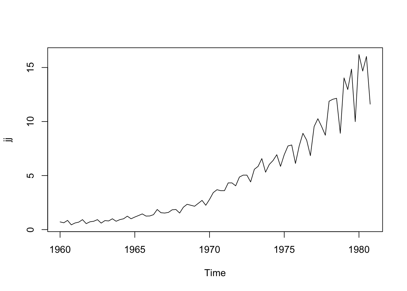
Below are the quarterly earnings per share of the company Johnson and Johnson from 1960-1980 in the astsa package (Stoffer 2025). The first observation is the 1st quarter of 1960 (\(t=1\)) and the second is the 2nd quarter of 1960 (\(t=2\))
plot(jj) # plot() is smart enough to make the right x-axis because jj is ts object
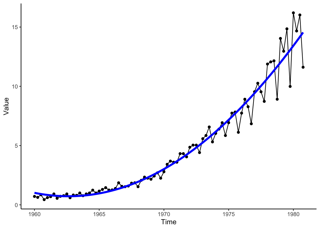
We see that the earnings are overall increasing over time, but a bit faster than a linear relationship (there is some curvature in the trend). Let’s transform this dataset into a data frame to use ggplot2, an alternative graphing package in R.
library(ggplot2)library(dplyr)jjTS <-data.frame(Value =as.numeric(jj), Time =time(jj), # time() works on ts objectsQuarter =cycle(jj)) # cycle() works on ts objectsquadTrendMod <-lm(Value ~poly(Time, degree =2, raw =TRUE), data = jjTS) # poly() fits a polynomial trend modeljjTS <- jjTS %>%mutate(Trend =predict(quadTrendMod)) # Add the estimated trend to the datasetjjTS %>%ggplot(aes(x = Time, y = Value)) +geom_point() +geom_line() +geom_line(aes(x = Time, y = Trend), color ='blue', size =1.5) +theme_classic()
Warning: Using `size` aesthetic for lines was deprecated in ggplot2 3.4.0.
ℹ Please use `linewidth` instead.
Don't know how to automatically pick scale for object of type <ts>. Defaulting
to continuous.
Data Example 2
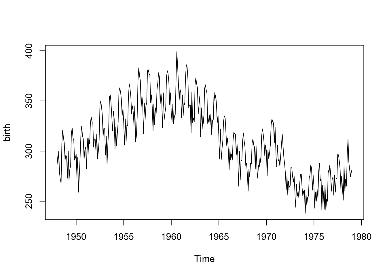
Below are the monthly counts (in thousands) of live births in the United States from 1948 to 1979. The first measurement is from January 1948 (\(t=1\)), then February 1948 (\(t=2\)), etc.
plot(birth) # plot() is smart enough to make the right x-axis because birth is ts object
Looking at the plot (time-ordered points are connected with a line segment), we note a positive linear relationship from about 1948 to 1960 and a somewhat negative relationship between 1960 to 1968, with another slight increase and then a drop around 1972. This is not a polynomial trend over time. We’ll need another approach!
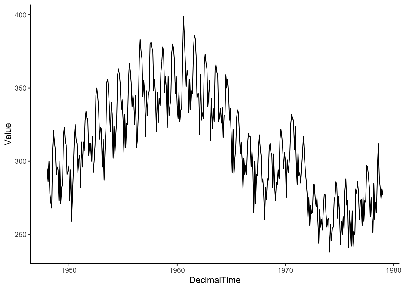
Let’s also transform this dataset into a data frame to use ggplot2.
birthTS <-data.frame(Year =floor(as.numeric(time(birth))), # time() works on ts objectsMonth =as.numeric(cycle(birth)), # cycle() works on ts objectsValue =as.numeric(birth))birthTS <- birthTS %>%mutate(DecimalTime = Year + (Month-1)/12)birthTS %>%ggplot(aes(x = DecimalTime, y = Value)) +geom_line() +theme_classic()
4.1.1.2 Splines
Let’s try a regression basis spline, which is a smooth piecewise polynomial. This means we break up the x-axis into intervals using knots or breakpoints and model a different polynomial in each interval. In particular, let’s fit a quadratic polynomial with knots/breaks at 1965 and 1972.
library(splines)TrendSpline <-lm(Value ~bs(DecimalTime, degree =2, knots =c(1965,1972)), data = birthTS)summary(TrendSpline)
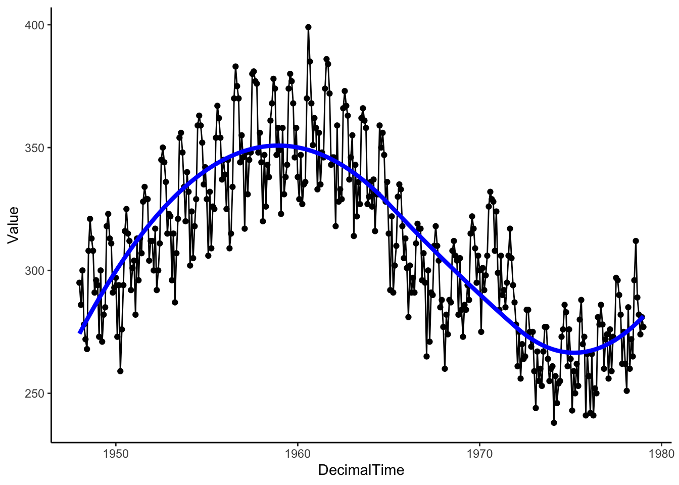
birthTS <- birthTS %>%mutate(SplineTrend =predict(TrendSpline))birthTS %>%ggplot(aes(x = DecimalTime, y = Value)) +geom_point() +geom_line() +geom_line(aes(x = DecimalTime, y = SplineTrend), color ='blue', size =1.5) +theme_classic()
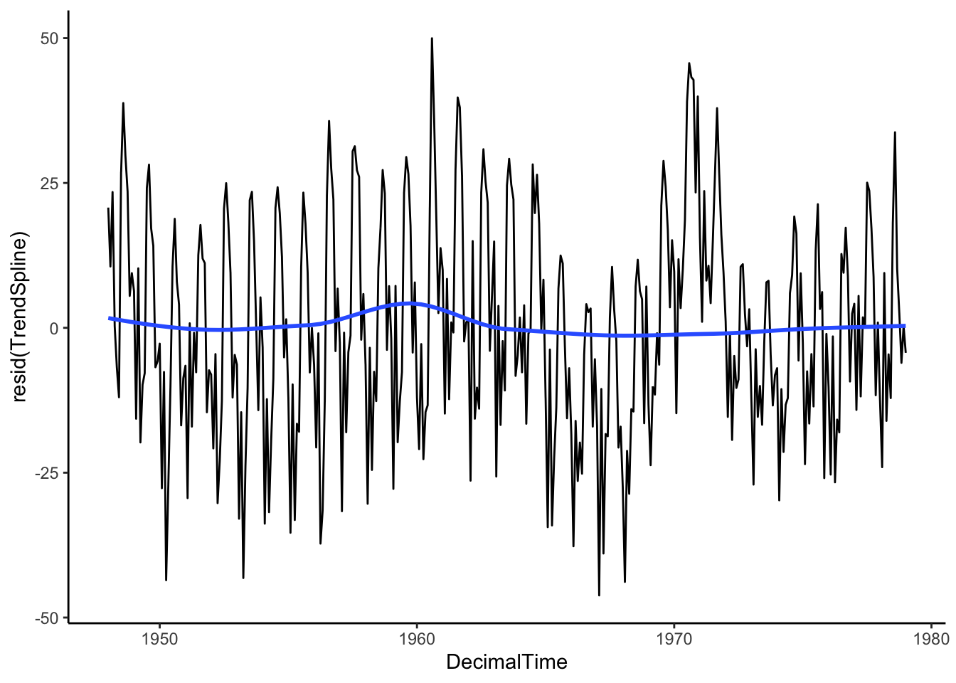
Then let’s see what is left over by plotting the residuals after removing the estimated trend. Is the mean constant? If so, we can ensure we’ve estimated and removed the long-range trend.
`geom_smooth()` using method = 'loess' and formula = 'y ~ x'
These parametric approaches give us an estimated function to plug in times and get a predicted trend value, but they might not quite pick up the full trend.
What are alternative methods for estimating non-linear trends?
4.1.2 Nonparametric Approaches
Nonparametric methods for estimating a trend use algorithms (steps of a process) rather than parametric functions (linear, polynomial, splines) with a finite number of parameters to estimate.
4.1.2.1 Local Regression
Have you ever wondered how geom_smooth() estimates that blue smooth curve?
If you look at the documentation for geom_smooth(), you’ll see that it uses the loess() function for smaller data sets. This trend estimation method is locally estimated scatterplot smoothing, also called local regression.
The loess algorithm is to predict the outcome (estimate the trend) at a point on the x-axis, \(x_0\), following the steps below:
Distance: calculate the distance between \(x_0\) and each observed points \(x\), \(d(x,x_0)=|x-x_0|\).
Find Local Area: keep the closest \(s\) proportion of observed data points (\(s\) determined by span parameter)
Fit Model: fit a linear or quadratic regression model to the local area, weighting points close to \(x_0\) higher (weighting determined by a chosen weighting kernel function)
Predict: use that local model to predict the outcome at \(x_0\)
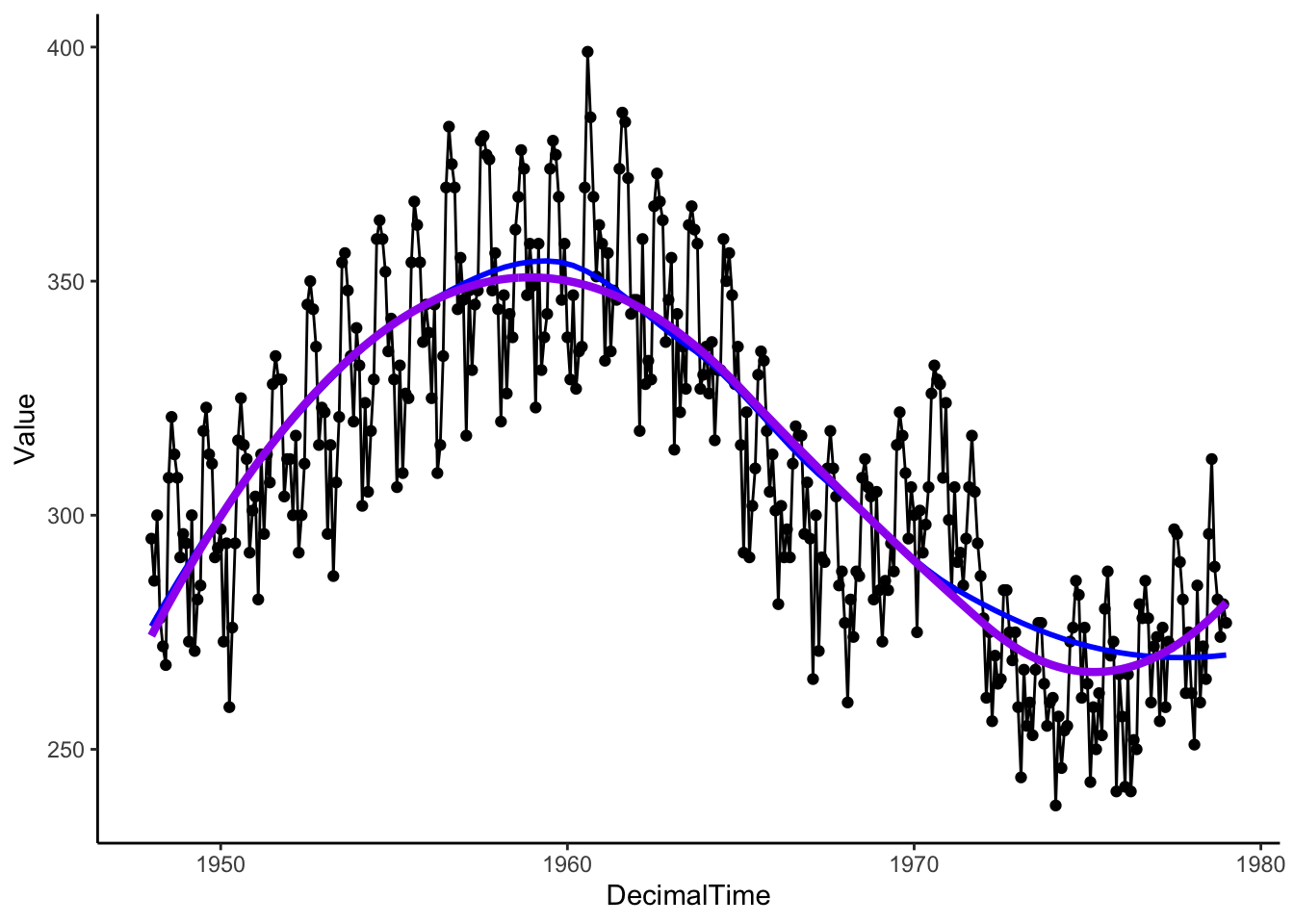
That process is repeated for a sequence of values along the x-axis to make a plot like the one below (blue: loess, purple: spline).
birthTS %>%ggplot(aes(x = DecimalTime, y = Value)) +geom_point() +geom_line() +geom_smooth(se =FALSE, color ='blue') +# uses loessgeom_line(aes(x = DecimalTime, y = SplineTrend), color ='purple', size =1.5) +theme_classic()
`geom_smooth()` using method = 'loess' and formula = 'y ~ x'
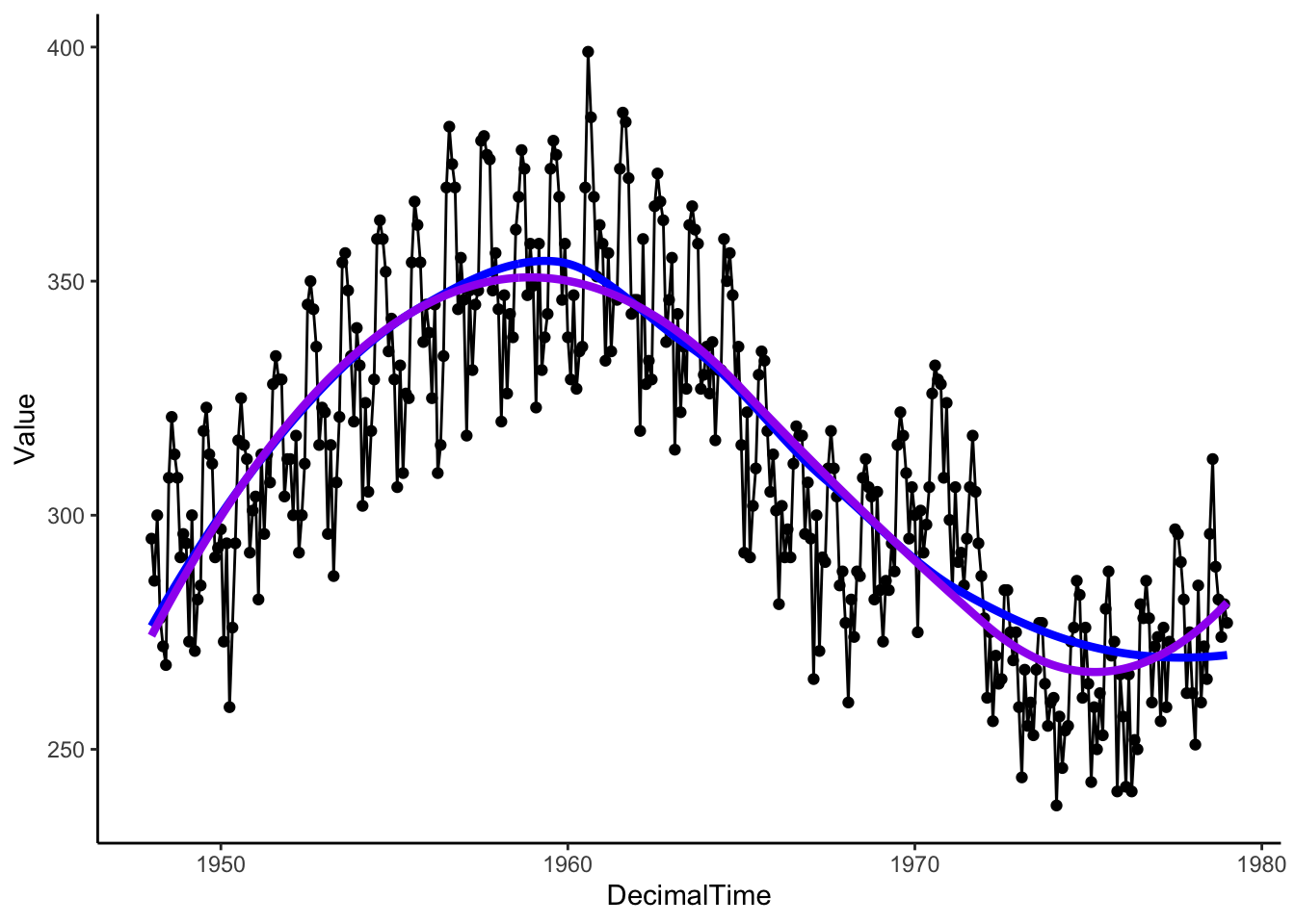
We can also get the estimated trend with the loess() function.
# Running loess separatelyLocalReg <-loess(Value ~ DecimalTime, data = birthTS, span = .75)birthTS <- birthTS %>%mutate(LoessTrend =predict(LocalReg))birthTS %>%ggplot(aes(x = DecimalTime, y = Value)) +geom_point() +geom_line() +geom_line(aes(x = DecimalTime, y = LoessTrend), color ='blue', size =1.5) +geom_line(aes(x = DecimalTime, y = SplineTrend), color ='purple', size =1.5) +theme_classic()
`geom_smooth()` using method = 'loess' and formula = 'y ~ x'
4.1.2.2 Moving Average Filter
Local regression is an extension of a simple idea called a moving average filter(See Chatfield and Xing 2019 for a brief introduction to moving averages and linear filtering in general).
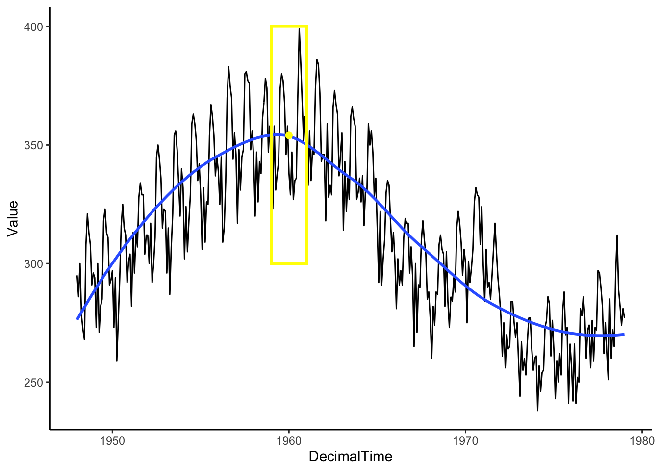
Imagine a window that only shows you what is “local” or right in front of you, and we can adjust the window width to include more or less data. In the illustration below, we have drawn a 2-year window around January 1960. When considering information around Jan 1960, the window limits our view to only those one year before and one year after (from Jan 1959-Jan 1961).
`geom_smooth()` using method = 'loess' and formula = 'y ~ x'
For our circumstances, the “local” window will include an odd number of observations (number of points = \(1+2a\) for a given \(a\) value). Among that small local group of observations, we take the average to estimate the mean at the center of those points (rather than fit a linear regression model),
`geom_smooth()` using method = 'loess' and formula = 'y ~ x'
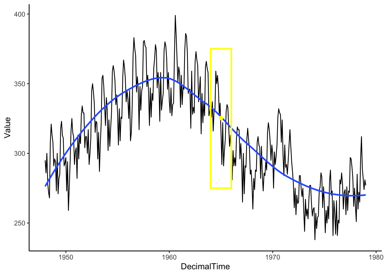
Then, we move the window and calculate the mean within that window. Continue until you have a smooth curve estimate for each point in the time range of interest.
Box <-data.frame(x =1965, y =325, w =2) #2-year window around 1980Mean <- birthTS %>%filter(DecimalTime <1965+1& DecimalTime >1965-1) %>%summarize(M =mean(Value)) %>%#Mean value of points in the windowmutate(x =1965)birthTS %>%ggplot(aes(x = DecimalTime, y = Value)) +geom_line() +geom_smooth(se =FALSE) +geom_tile(data = Box, aes(x = x,y=y,width=w),height =100, fill=alpha("grey",0), colour ='yellow',size =1) +geom_point(data = Mean, aes(x = x, y = M), colour ='yellow', size =2)+theme_classic()
`geom_smooth()` using method = 'loess' and formula = 'y ~ x'
This method works well for windows of odd-numbered length (equal number of points around the center), but it can be adjusted if you desire an even-numbered length window by adding 1/2 of the two extreme lags so that the middle value lines up with time \(t\).
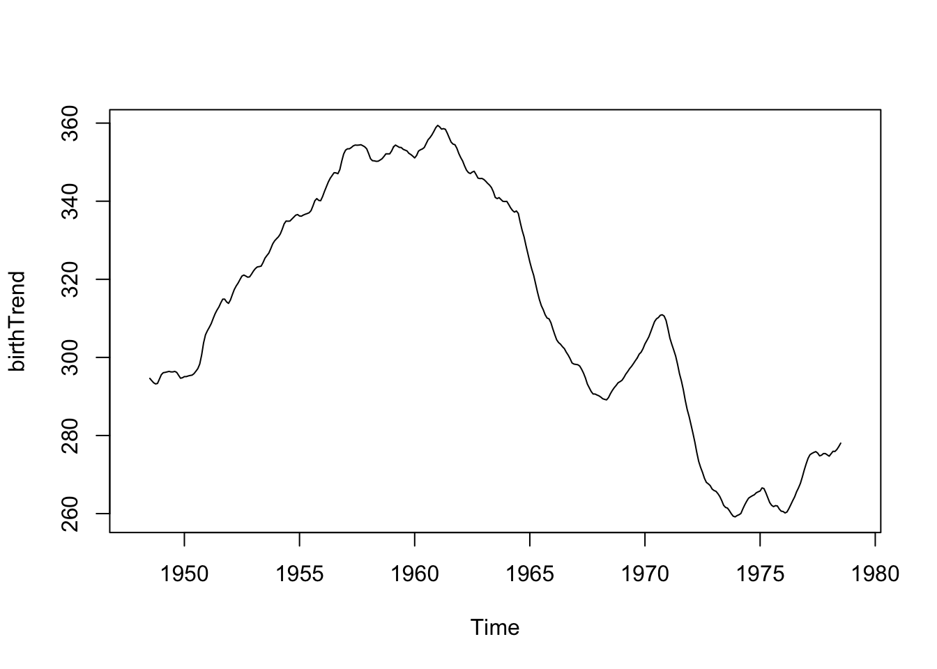
For the above monthly data example, we might want a 12-point moving average, so we would have
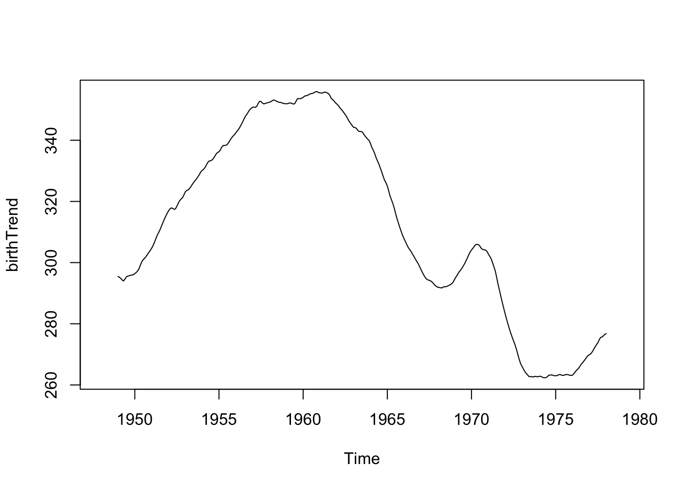
fltr <-c(0.5, rep(1, 11), 0.5)/12# weights for the weighted average abovebirthTrend <- stats::filter(birth, filter = fltr, method ='convo', sides =2) #use the ts object rather than the data frameplot(birthTrend)
Now, if we increase the window’s width (24-point moving window), you should see a smoother curve.
fltr <-c(0.5, rep(1, 23), 0.5)/24# weights for moving averagebirthTrend <- stats::filter(birth, filter = fltr, method ='convo', sides =2) # use the ts object rather than the data frameplot(birthTrend)
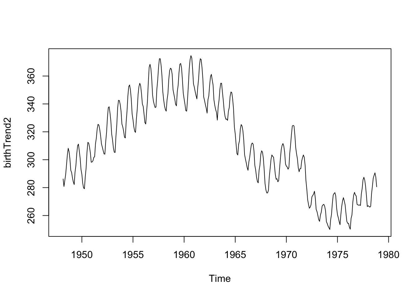
What if we did a 5-point moving average instead of a 12 or 24-point moving average?
We see the seasonality (repeating cycles) because the 5-point window averages about half of the year’s data for each estimate. Thus, the highs and lows don’t balance each other out.
You must be mindful of the window width for the moving average, depending on the context of the data and the existing cycles in the data.
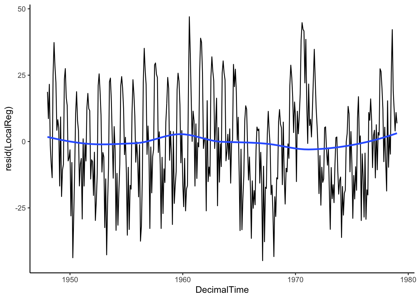
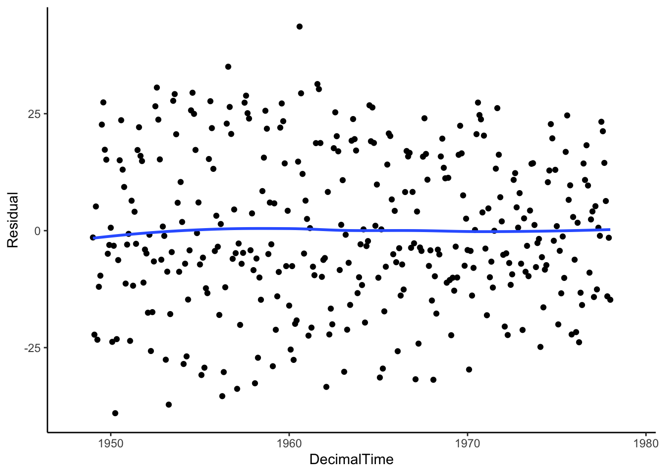
Let’s see what is left over. Is the mean of the residuals constant across time (indicating that we have fully removed the trend)?
Don't know how to automatically pick scale for object of type <ts>. Defaulting
to continuous.
`geom_smooth()` using method = 'loess' and formula = 'y ~ x'
Warning: Removed 24 rows containing non-finite outside the scale range
(`stat_smooth()`).
Warning: Removed 24 rows containing missing values or values outside the scale range
(`geom_point()`).
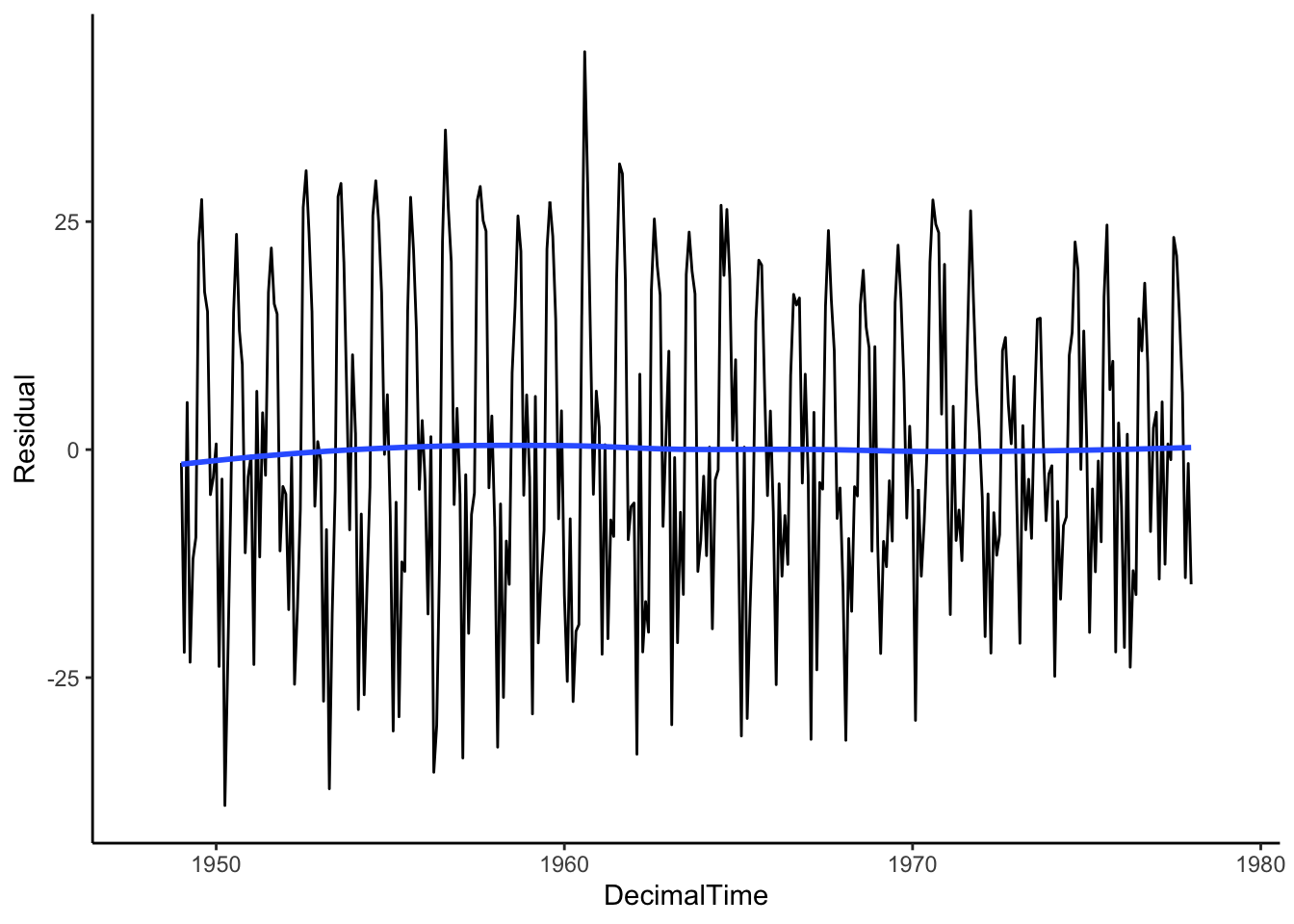
If we connect the points, we might see a cyclic pattern…
Don't know how to automatically pick scale for object of type <ts>. Defaulting
to continuous.
`geom_smooth()` using method = 'loess' and formula = 'y ~ x'
Warning: Removed 24 rows containing non-finite outside the scale range
(`stat_smooth()`).
Warning: Removed 24 rows containing missing values or values outside the scale range
(`geom_line()`).
We still have to deal with seasonality (we’ll get there), but the moving average does a fairly good job at removing the trend because we see that the trend of the residuals is 0 on average!
The moving average filter did a decent job of estimating the trend because of its flexibility, but we can’t write down a function statement for that trend. This is the downside of nonparametric methods.
4.1.2.3 Differencing to Remove Trend
If we don’t necessarily care about estimating the trend for prediction, we could use differencing to explicitly remove a trend.
We’ll talk about first and second-order differences, which are applicable if we have a linear or quadratic trend.
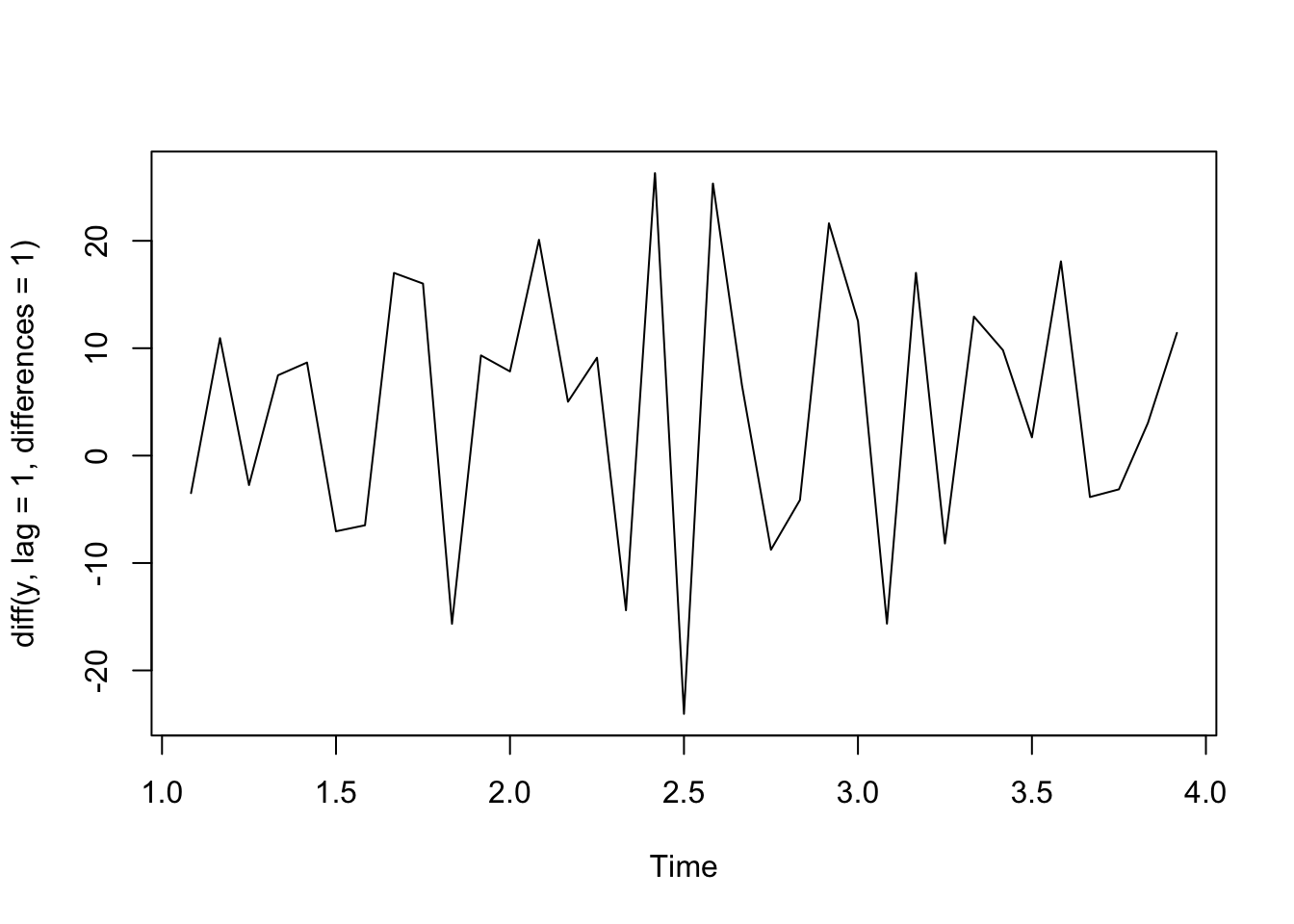
Linear Trend - First Difference
If we have a linear trend such that \(Y_t = b_0 + b_1 t + \epsilon_t\), the difference between neighboring outcomes (1 time unit apart) will essentially remove that trend.
Take the outcome at time \(t\) and an outcome that lags behind one time unit:
\[Y_t - Y_{t-1} = (b_0 + b_1 t + \epsilon_t) - (b_0 + b_1 (t-1) + \epsilon_{t-1})\]\[= b_0 + b_1 t + \epsilon_t - b_0 - b_1t + b_1 - \epsilon_{t-1}\]\[= b_1 + \epsilon_t - \epsilon_{t-1}\] which is constant with respect to time, \(t\).
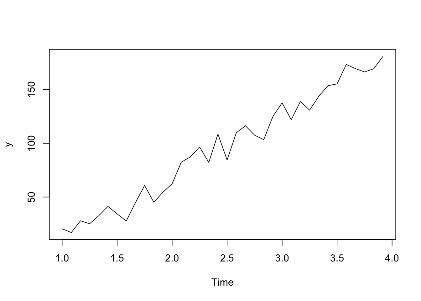
See below for a simulated example.
t <-1:36y <-ts(2+5*t +rnorm(36,sd =10), frequency=12)plot(y)
plot(diff(y, lag =1, differences =1))
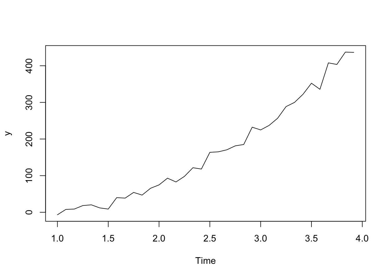
Quadratic Trend - Second Order Differences
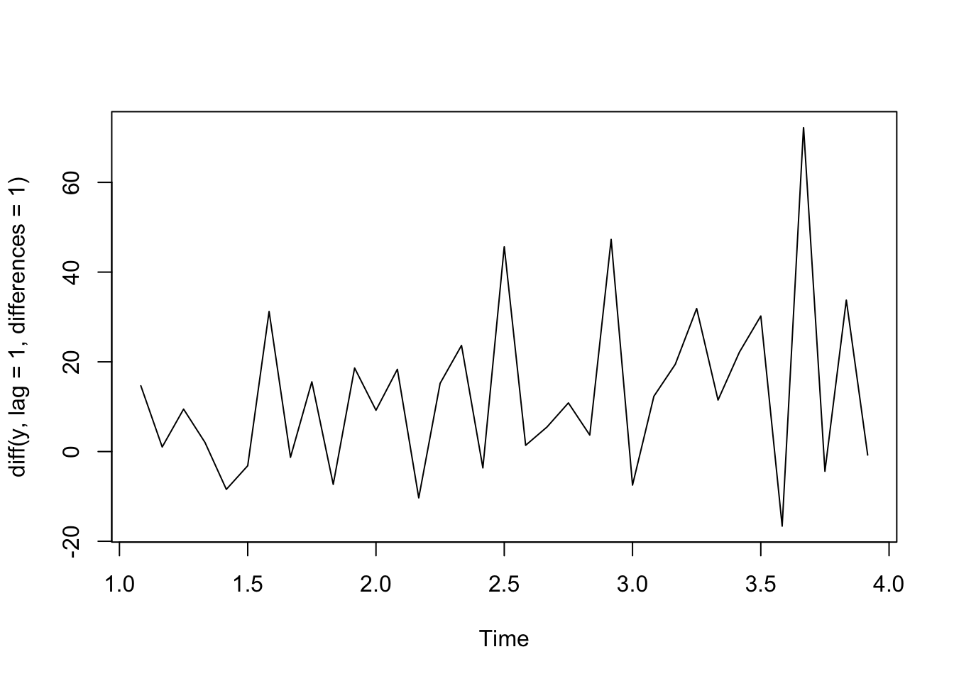
If we have a quadratic relationship such that \(Y_t = b_0 + b_1 t+ b_2 t^2 + \epsilon_t\), then taking the second order difference between neighboring outcomes will remove that trend.
Take the outcome at time \(t\) and an outcome that lags behind one time unit (first difference): \[(Y_t - Y_{t-1}) = (b_0 + b_1 t+ b_2 t^2 + \epsilon_t) - (b_0 + b_1 (t-1)+ b_2 (t-1)^2 + \epsilon_{t-1})\]\[= b_0 + b_1 t + b_2 t^2 + \epsilon_t - b_0 - b_1 x_t + b_1 - b_2 t^2 + 2b_2t - b_2^2 - \epsilon_{t-1}\]\[= b_1- b_2^2 + 2b_2t + \epsilon_t - \epsilon_{t-1}\] and thus, the second-order difference is the difference in the neighboring first differences:
\[(Y_t - Y_{t-1}) - (Y_{t-1} - Y_{t-2}) = (b_1- b_2^2 + 2b_2t + \epsilon_t - \epsilon_{t-1}) - (b_1- b_2^2 + 2b_2(t-1) + \epsilon_{t-1} - \epsilon_{t-2})\]\[= 2b_2 + \epsilon_t - 2\epsilon_{t-1} + \epsilon_{t-2}\] which is constant with respect to time, \(t\).
See below for an example of simulated data.
t <-1:36y <-ts(2+1.5*t + .3*t^2+rnorm(36,sd =10), frequency=12)plot(y)
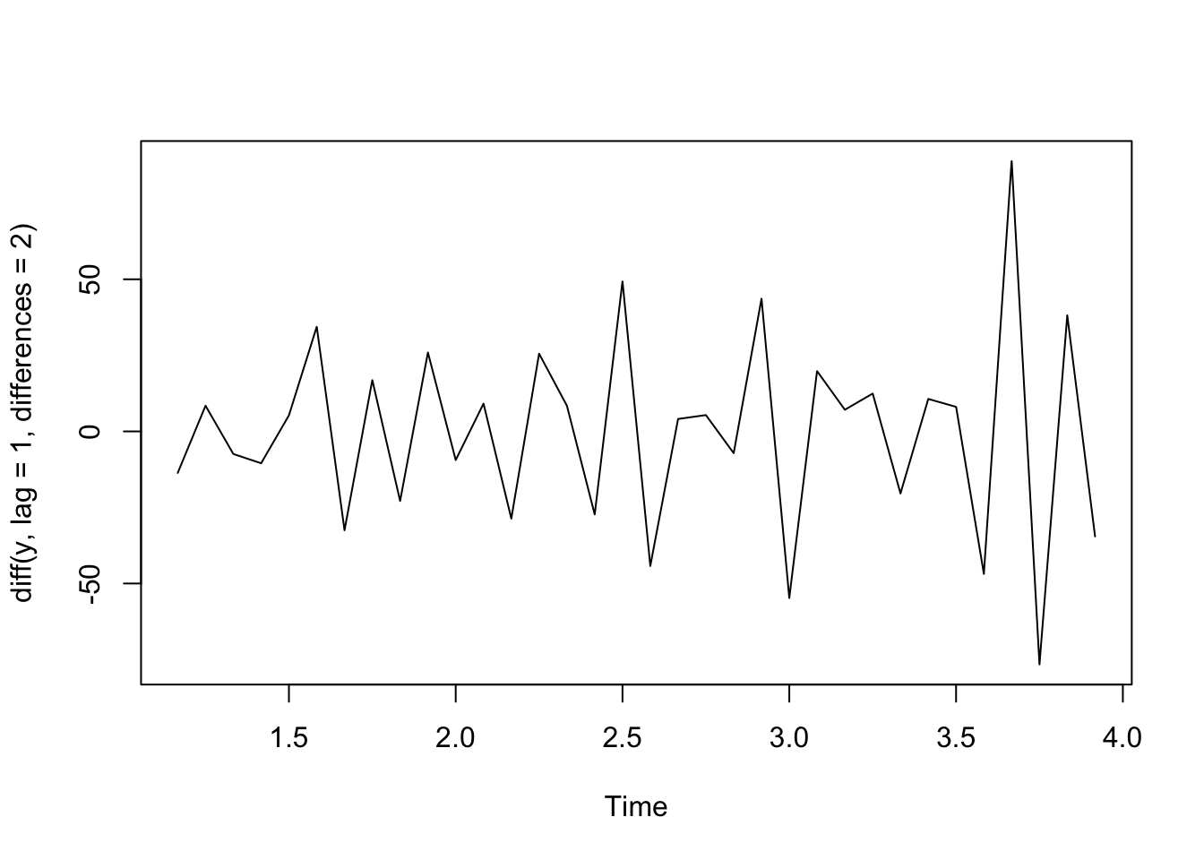
plot(diff(y, lag =1, differences =1)) #first difference
plot(diff(y, lag =1, differences =2)) #second order difference
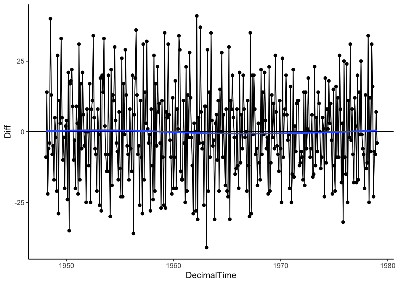
Let’s see what we get when we use differencing on the real birth count data. It looks like the first differences resulted in data with no overall trend despite the complex trend over time!
`geom_smooth()` using method = 'loess' and formula = 'y ~ x'
Warning: Removed 1 row containing non-finite outside the scale range
(`stat_smooth()`).
Warning: Removed 1 row containing missing values or values outside the scale range
(`geom_point()`).
Warning: Removed 1 row containing missing values or values outside the scale range
(`geom_line()`).
4.1.3 In Practice: Estimate vs. Remove
We have a few methods to estimate the trend,
Parametric Regression: Global Transformations (polynomials)
Parametric Regression: Spline basis
Nonparametric: Local Regression
Nonparametric: Moving Average Filter
Among the estimation methods, two are parametric in that we estimate slope parameters or coefficients (regression techniques), and two are nonparametric in that we do not have any parameters to estimate but rather focus on the whole function.
Things to consider when choosing an estimation method:
How well does it approximate the true underlying trend? Does it systematically under- or overestimate the trend for certain periods, or are the residuals on average zero across time?
Do you want to use past trends to predict the future? If so, you may want to consider a parametric approach.
We have two approaches to removing the trend,
Estimate, then Residuals. Estimate the trend first, then subtract the trend from observations to get residuals, \(y_t - \hat{f}(x_t)\).
Difference. Skip the estimating and try first or second-order differencing of neighboring observations.
Things to consider when choosing an approach for removing the trend:
How well does it remove the underlying trend? Are the residuals (what is left over) close to zero on average, or are there still long-range patterns in the data?
Do you want to report on the estimated trend? Then estimate first.
If your main goal is prediction, try differencing.
4.2 Seasonality
Once we’ve estimated and removed the trend, we may notice cyclic patterns left in the data. Depending on the cyclic pattern’s form, we could use a few different techniques to model the seasonal pattern.
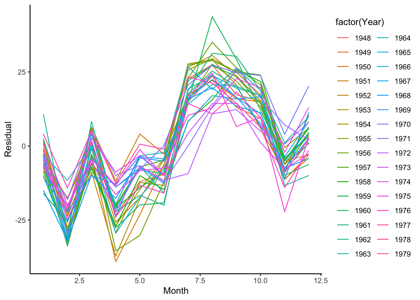
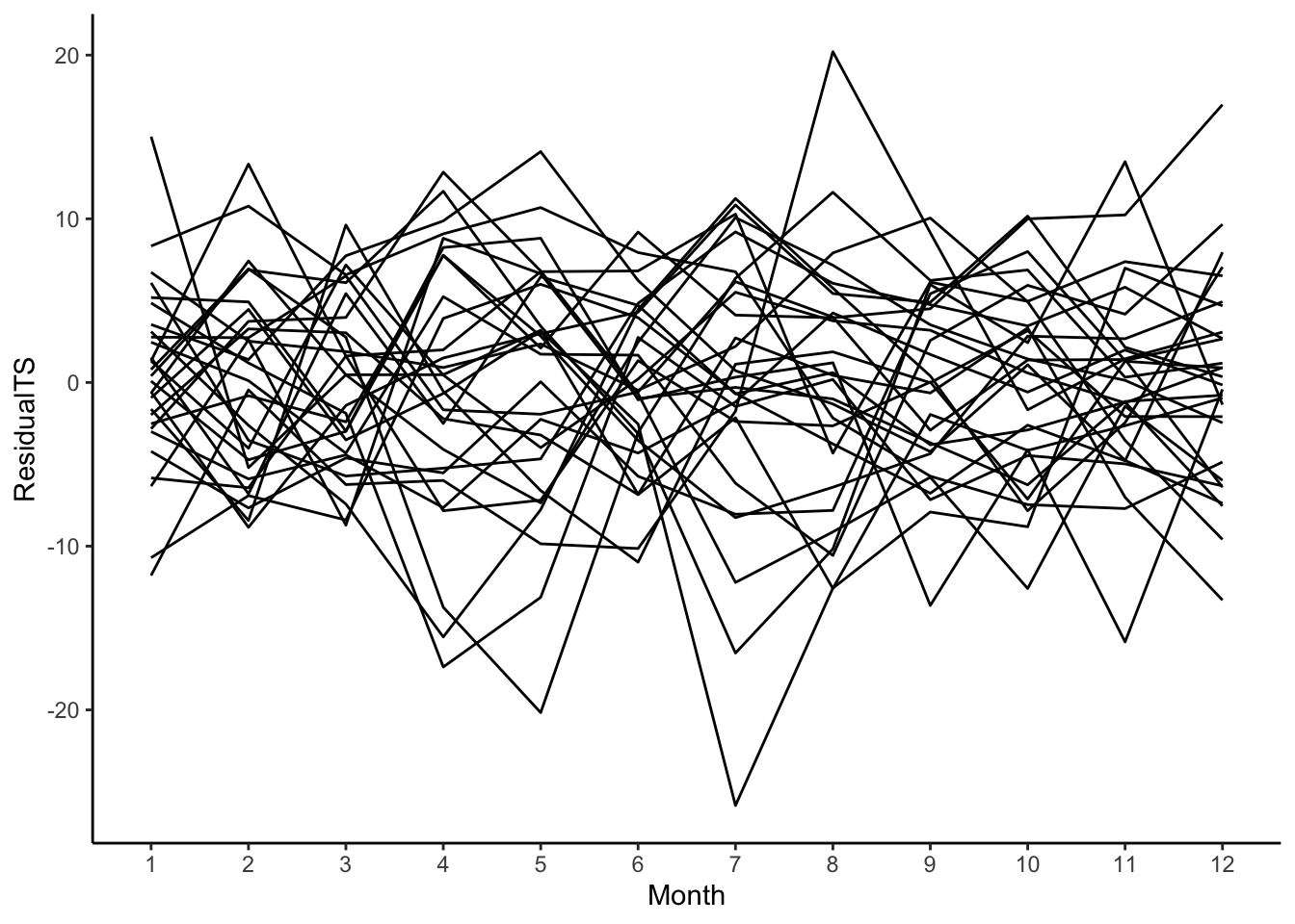
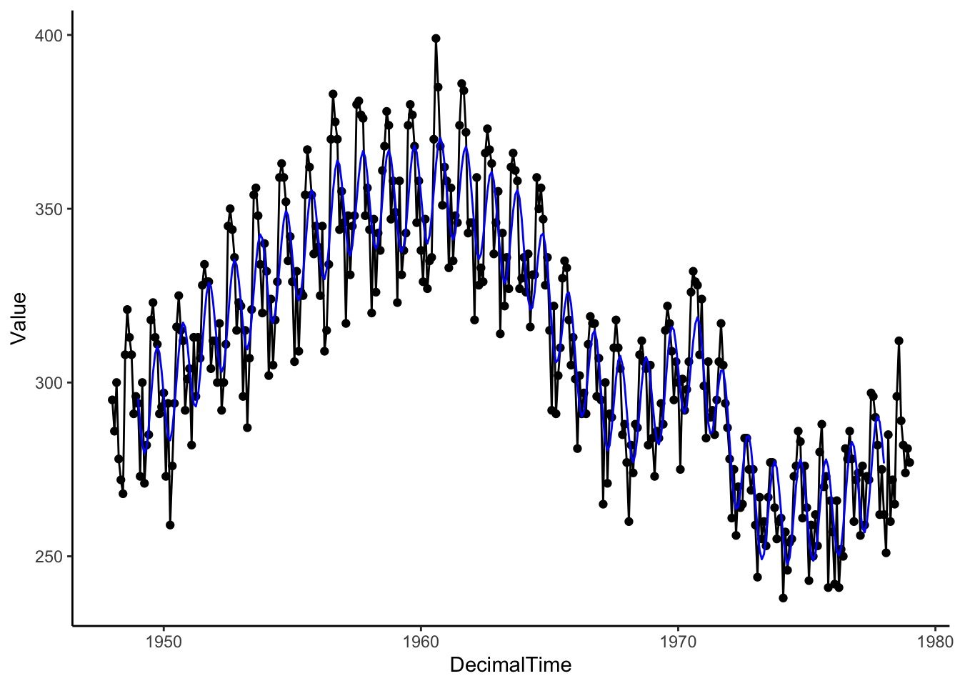
First, let’s visualize the variability in the seasonality between different years for the birth data set to see if there is a consistent cycle. To do so, we’ll work with the residuals after removing the trend (for now, let’s use the moving average filter). Since we are interested in the cycles, we want to know how the number of births varies across the months within a year.
Using the ggplot2 package, we can visualize this with geom_line() by plotting the residuals by the month and having it color each line according to the year. To do this, it creates one line per year. Interestingly, August and September have the highest residuals (approximately nine months after winter break). In this case, we see that every year follows the same pattern.
birthTS %>%ggplot(aes(x = Month, y = Residual, color =factor(Year))) +geom_line() +theme_classic()
Don't know how to automatically pick scale for object of type <ts>. Defaulting
to continuous.
Warning: Removed 24 rows containing missing values or values outside the scale range
(`geom_line()`).
4.2.1 Parametric Approaches
Similar to the trend, we can use some of our parametric tools to model the cyclic patterns in the data using our linear regression structures.
4.2.1.1 Indicator Variables
To estimate the seasonality that does not have a recognizable cyclic functional pattern (sine or cosine curve), we can model each month (or appropriate time unit within a cycle) to have its own average by including indicator variables for each month (or appropriate unit within a cycle) in a linear regression model.
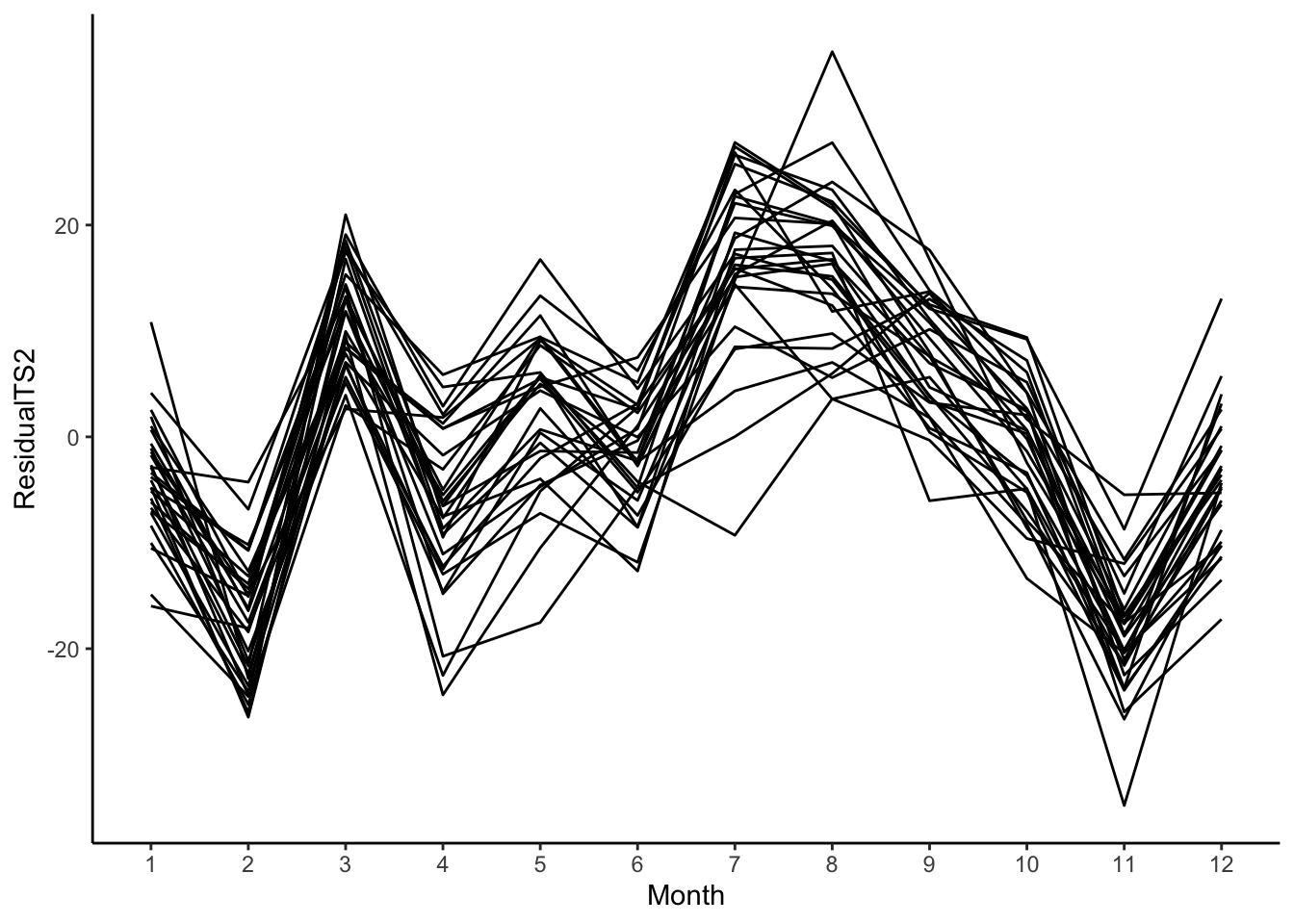
Like when we estimate the trend, we want to ensure that we have fully estimated the seasonality, but check the residuals to ensure that there is no seasonality in what is left over.
Don't know how to automatically pick scale for object of type <ts>. Defaulting
to continuous.
`geom_smooth()` using method = 'loess' and formula = 'y ~ x'
Warning: Removed 24 rows containing non-finite outside the scale range
(`stat_smooth()`).
Removed 24 rows containing missing values or values outside the scale range
(`geom_line()`).
4.2.1.2 Sine and Cosine Curves
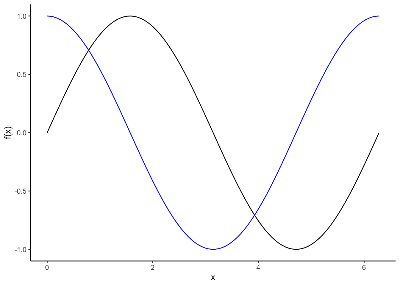
While it isn’t the case for this birth data set, if the cyclic pattern is like a sine curve, we could use a sine or cosine curve to model the relationship.
time <-seq(0,2*pi,length =100)tibble(t = time,sin =sin(time),cos =cos(time)) %>%ggplot(aes(x = t, y = sin)) +geom_line() +geom_line(aes(x = t, y = cos),color ='blue') +labs(x ='x',y ='f(x)') +theme_classic()
The period (length of 1 full cycle) of a sine or cosine function is \(2\pi\)
We can write a sine curve model as \(A\sin(2\pi ft + s)\) where \(A\) is the amplitude (peak deviation from 0 instead of 1), \(f\) is the frequency (number of cycles that occur each unit of time), \(t\) is the time, and \(s\) is the shift in the x-axis.
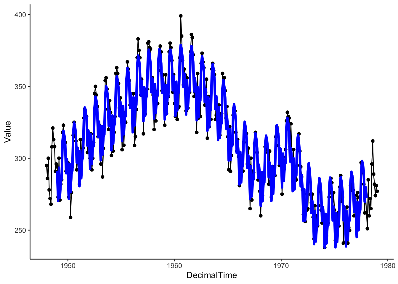
Now, let’s try to apply it to the birth data.
SineSeason <-lm(Residual ~sin(2*pi*(DecimalTime) ), data = birthTS) # frequency is one because a unit in DecimalTime is one yearSineSeason
Call:
lm(formula = Residual ~ sin(2 * pi * (DecimalTime)), data = birthTS)
Coefficients:
(Intercept) sin(2 * pi * (DecimalTime))
-0.04286 -14.61751
# Estimate Trend + SeasonalitybirthTS %>%mutate(SeasonSine =predict(SineSeason, newdata =data.frame(DecimalTime = birthTS$DecimalTime))) %>%ggplot(aes(x = DecimalTime, y = Value)) +geom_point() +geom_line() +geom_line(aes(x = DecimalTime, y = Trend + SeasonSine), color ='blue') +theme_classic()
Warning: Removed 24 rows containing missing values or values outside the scale range
(`geom_line()`).
Don't know how to automatically pick scale for object of type <ts>. Defaulting
to continuous.
`geom_smooth()` using method = 'loess' and formula = 'y ~ x'
Warning: Removed 24 rows containing non-finite outside the scale range
(`stat_smooth()`).
Removed 24 rows containing missing values or values outside the scale range
(`geom_line()`).
Since we still see a pattern in these residuals, using a sine/cosine curve is not an accurate way to estimate the cyclic pattern in this particular data set.
Data Example 3
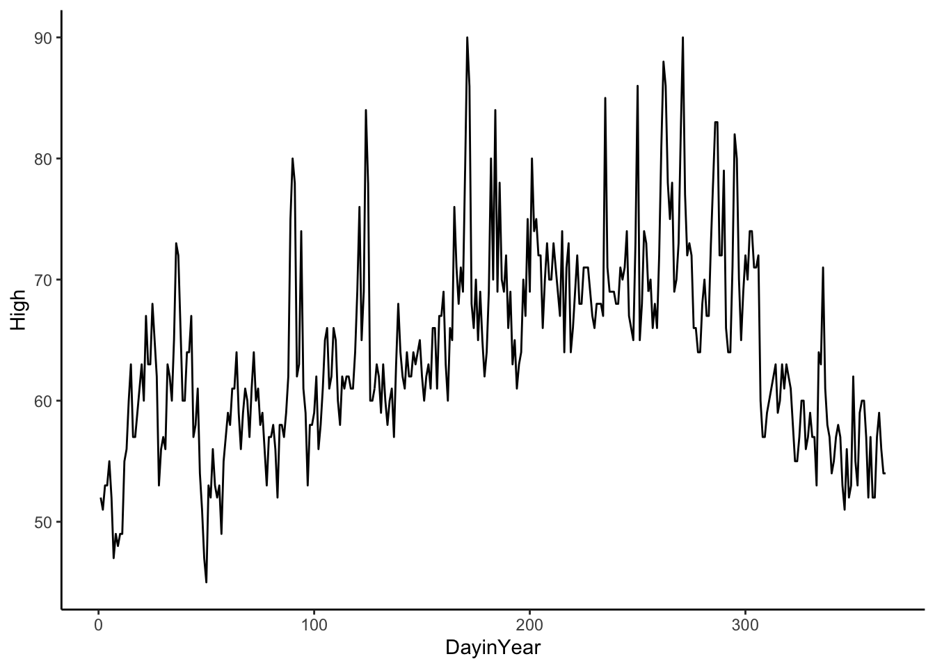
Here is the daily temperature data in San Francisco in 2011. We only have one year, but we can see that the cycle shape is closer to a cosine curve. The period, the length of one cycle, of a cosine or sine curve is \(2*\pi\), so we need to adjust the period when we fit a cosine or sine curve to our data. In the case below, the period is 365 since our time variable is DayinYear, where 1 unit is one day in the year (Jan 1 is one and Dec 31 is 365).
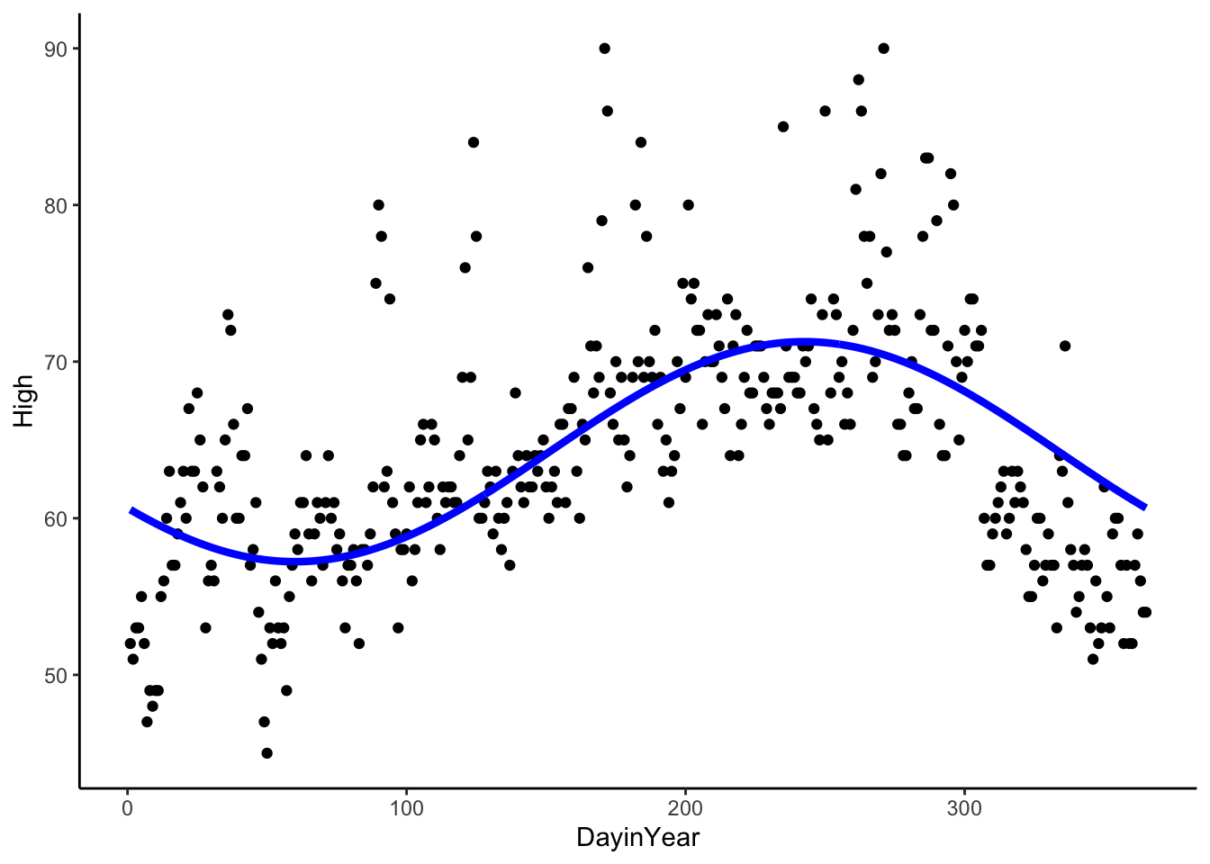
CosSeason <-lm(High ~cos(2*pi*(DayinYear-60)/365), data = sfoWeather) # frequency is 1/365 because a unit in DayinYear is 1 dayCosSeason
Call:
lm(formula = High ~ cos(2 * pi * (DayinYear - 60)/365), data = sfoWeather)

Coefficients:
                       (Intercept)  cos(2 * pi * (DayinYear - 60)/365)
                            64.249                              -7.022
sfoWeather %>%mutate(Season =predict(CosSeason)) %>%ggplot(aes(x = DayinYear, y = High)) +geom_point() +geom_line(aes(x = DayinYear, y = Season), color ='blue', size =1.5) +theme_classic()
To recap:
For a cosine function,
\[A\cos(Bx + C) + D\]
the period is \(\frac{2*\pi}{|B|}\), the amplitude is \(A\) (the coefficient in our linear model), the phase shift is \(C\) (included in our model above) and the vertical shift is \(D\) (intercept in our linear model).
4.2.2 Nonparametric Approaches
Similar to the trend, we could use local regression or moving averages to estimate the trend and seasonality as long as we define the local area small enough to pick up the cycles.
The disadvantage of this approach is that we will not be able to use the estimate to make predictions in the future because we do not learn general patterns of trend and seasonality.
4.2.2.1 Differencing to Remove Seasonality
Like removing a trend, we can use differencing to remove seasonality if we don’t need to estimate it. Rather than a difference between neighboring observations, we will take differences between observations that are approximately one period apart. The period, length of one cycle, is \(k\) observations such that \(y_t\) is similar to \(y_{t-k}\) and \(y_{t-2k}\), then we’ll take differences between observations that are \(k\) observations apart.
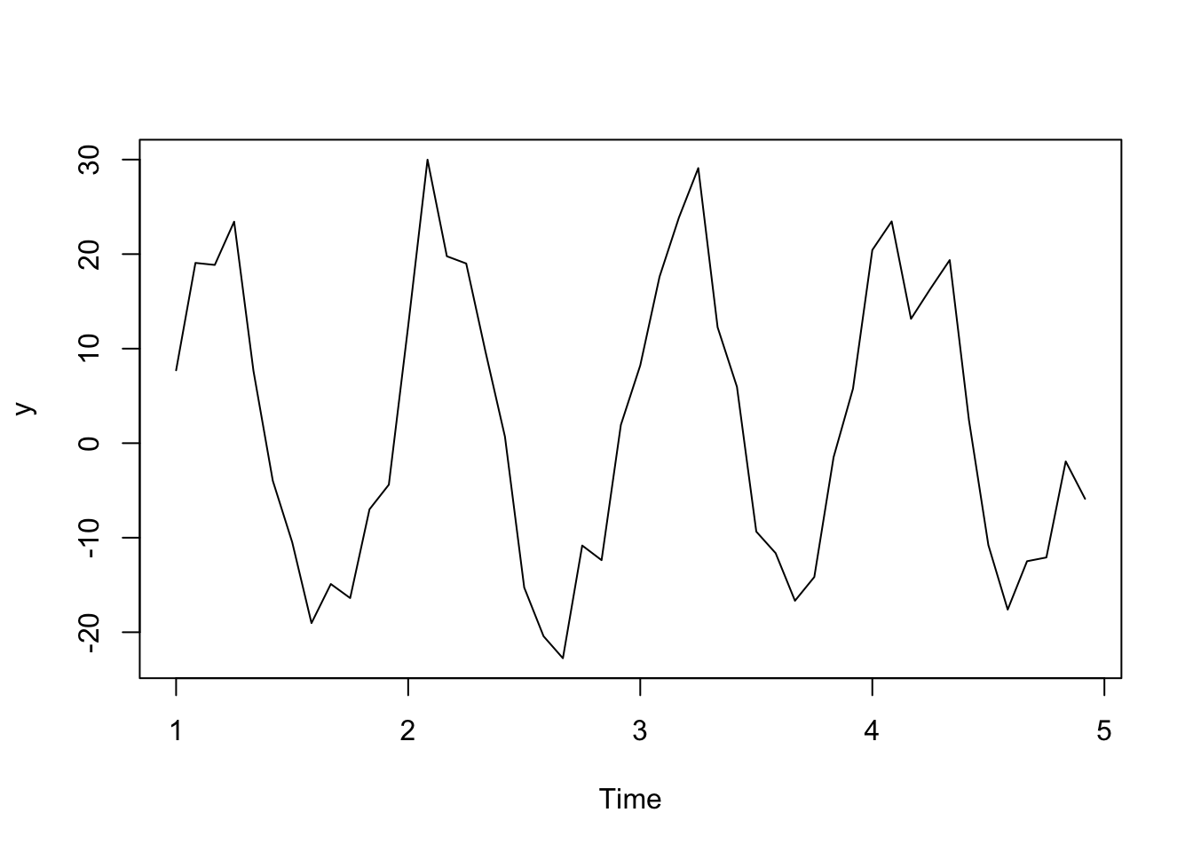
For example, if you have monthly data and an annual cycle, you’d want to take differences between observations that are 12 lags apart (12 months apart). See the simulated monthly data below.
t <-1:48y <-ts(2+20*sin(2*pi*t/12) +rnorm(48,sd =5), frequency=12)plot(y)
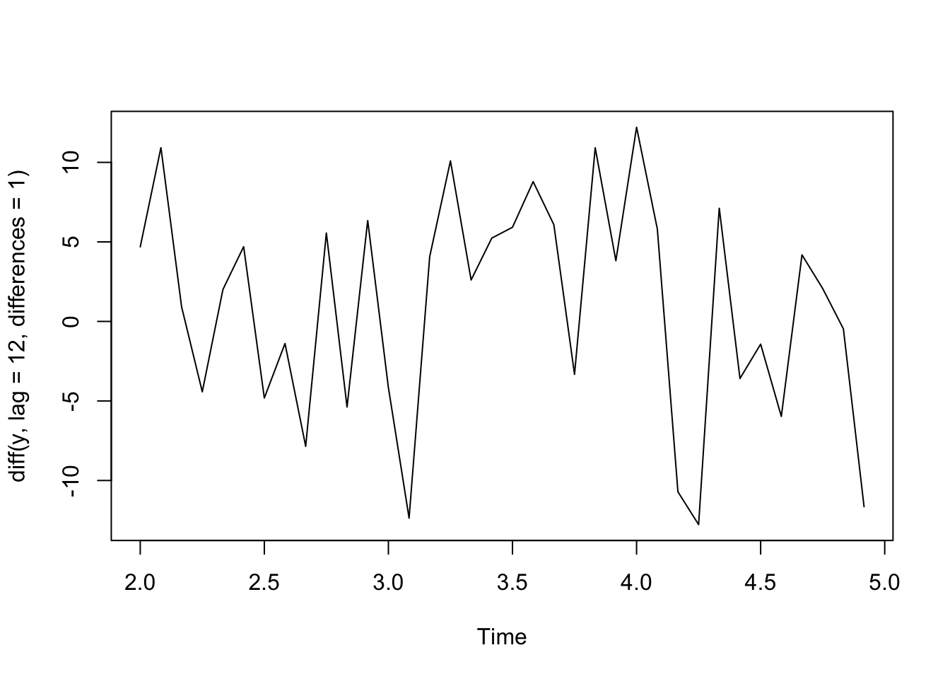
plot(diff(y, lag =12, differences =1)) #first order difference of lag 12
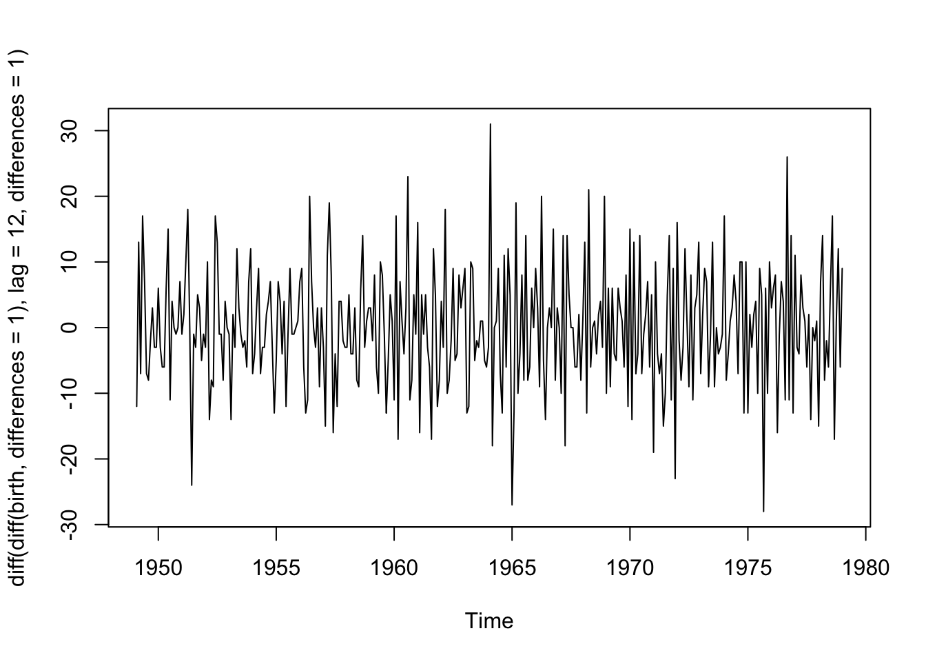
Let’s try this approach with the birth data since we saw annual seasonality by month. First, we take first differences of neighboring values to remove the trend. Then we’ll take the first differences of lag 12 to remove the seasonality. No obvious trends or seasonality remain in the data, and it is centered around 0.
plot(diff(diff(birth,differences =1), lag =12, differences =1))
What is left over, the random errors, are what we need to worry about now.
We’ll first talk about how we might model the errors from time series data and then talk about translating these ideas to other types of correlated data.
Chatfield, Chris, and Haipeng Xing. 2019. The Analysis of Time Series: An Introduction with r. Chapman; Hall/CRC.