acf(birth) # acf works well on ts objects (lag 1.0 is one year since it knows that one year is one cycle)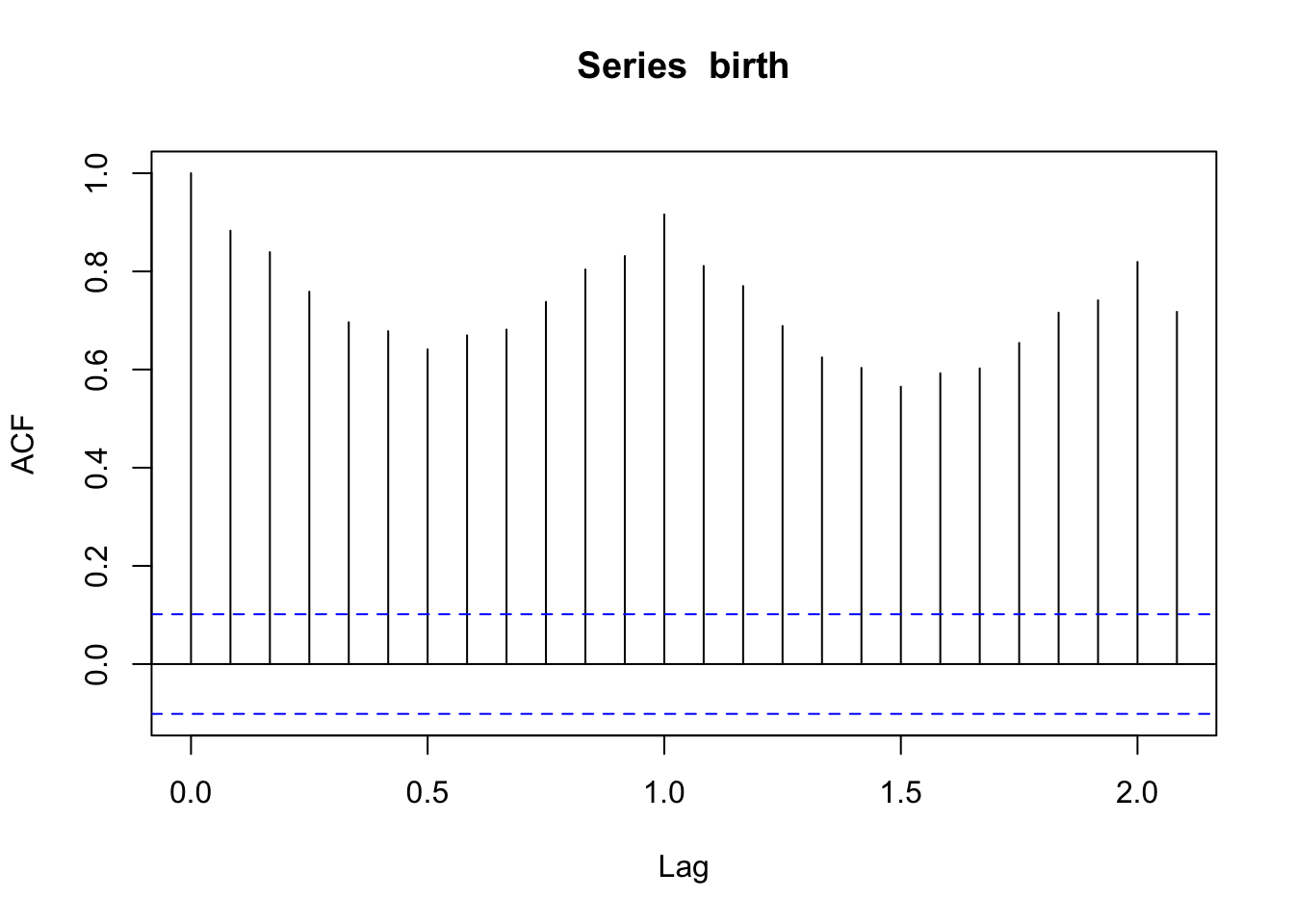
We will start with univariate time series, which is defined as a sequence of measurements of the same characteristic collected over time at regular intervals. We’ll notate this time series as
\[y_t\text{, for } t = 1,2,...,n\]
where \(t\) indexes time in a chosen unit.
For example, if data are collected yearly, \(t=1\) indicates the first year, etc. If data are collected every day, then \(t=1\) indicates the first day of data collection. In other settings, we may have monthly or hourly measurements such that \(t\) indices months or hours from the beginning of the study period.
There are two main approaches to analyzing time series data: time-domain and frequency-domain analysis. In this class, we’ll focus on the time-domain analysis. For frequency domain approaches, check out the Other Time Series References.
As you’ve seen, R has a special format (an object class) for time series data called a ts object. If the data are not already in that format, you can create a ts object with the ts() function. Besides the data, it requires two pieces of information.
The first is frequency. The name is a bit of a misnomer because it does not refer to the number of cycles per unit of time but rather the number of observations/samples per cycle.
We typically work with one day or one year as the cycle. So, if the data were collected each hour of the day, then frequency = 24. If the data is collected annually, frequency = 1; quarterly data should have frequency = 4; monthly data should have frequency = 12; weekly data should have frequency = 52.
The second piece of information is start, and it specifies the time of the first observation in terms of (cycle, frequency). In most use cases, it is (day, hour), (year, month), (year, quarter), etc. So, for example, if the data were collected monthly beginning in November of 1969, then frequency = 12 and start = c(1969, 11). If the data were collected annually, you specify start as a scalar (e.g., start = 1991) and omit frequency (i.e., R will set frequency = 1 by default).
This is a useful format for us because the plot.ts() or plot(ts()) functions will automatically correctly label the x-axis according to time. Additionally, there are special functions that work on ts objects such as decompose() that visualizes the basic decomposition of the series into trend, season, and error.
If you have multiple characteristics or variables measured over time, we could combine them in one ts object by considering the intersection (overlapping periods) with ts.intersect() or the union (all times) of the two time series with ts.union().
As you’ve seen above, it may also be useful to have data in a data.frame() format instead of a ts object if you want to use ggplot() or lm(). You should be familiar with both data formats to go back and forth as necessary.
As we discussed earlier, the key feature of correlated data is the covariance and correlation of the data. We have decomposed the data for time series into trend, seasonality, and noise or error. We will now work to model the dependence in the errors.
Remember: For a stationary random process, \(Y_t\) (constant mean, constant variance), the autocovariance function is only dependent on the different in time, which we will refer to as the lag \(h\), so
\[\Sigma(h) = Cov(Y_t, Y_{t+|h|}) = E[(Y_t - \mu_t)(Y_{t+|h|} - \mu_{t+|h|})] \] for any time \(t\).
Most time series are not stationary because they do not have a constant mean across time. By removing the trend and seasonality, we attempt to get errors (also called residuals) with a constant mean around 0. We’ll discuss the constant variance assumption later.
If we assume that the residuals, \(y_1,...,y_n\), are generated from a stationary process, we can estimate the autocovariance function with the sample autocovariance function (ACVF),
\[c_h = \frac{1}{n}\sum^{n-|h|}_{t=1}(y_t - \bar{y})(y_{t+|h|} - \bar{y})\] where \(\bar{y}\) is the sample mean, averaged across time, because we are assuming the mean is constant.
There are a few useful properties of the ACVF function. For any sequence of observations, \(y_1,...,y_n\),
The sample autocorrelation function (ACF) is the covariance divided by the variance, also known as the covariance for lag 0,
\[r_h = \frac{c_h}{c_0}\text{ for } c_0 > 0\]
There are a few useful properties of the ACF function. For any sequence of observations, \(y_1,...,y_n\),
We expect a fairly high correlation between observations with large lags for a non-stationary series with a trend and seasonality. This high correlation pattern typically indicates that you need to deal with trend and seasonality.
acf(birth) # acf works well on ts objects (lag 1.0 is one year since it knows that one year is one cycle)
We would like to see the autocorrelation of the random errors after removing the trend and the seasonality. Let’s look at the sample autocorrelation of the residuals from the model with a moving average filter estimated trend and monthly averages to account for seasonality.
birthTS <- data.frame(
  Year = floor(as.numeric(time(birth))), # time() works on ts objects
  Month = as.numeric(cycle(birth)), # cycle() works on ts objects
  Value = as.numeric(birth)) %>%
  mutate(DecimalTime = Year + (Month-1)/12)

fltr <- c(0.5, rep(1, 23), 0.5)/24 # weights for moving average
birthTrend <- stats::filter(birth, filter = fltr, method = 'convo', sides = 2) # use the ts object rather than the data frame

birthTS <- birthTS %>%
  mutate(Trend = birthTrend) %>%
  mutate(Residual = Value - Trend)
birthTS %>%
dplyr::select(Residual) %>%
dplyr::filter(complete.cases(.)) %>%
acf() # if the data is not a ts object, lags will be in terms of the index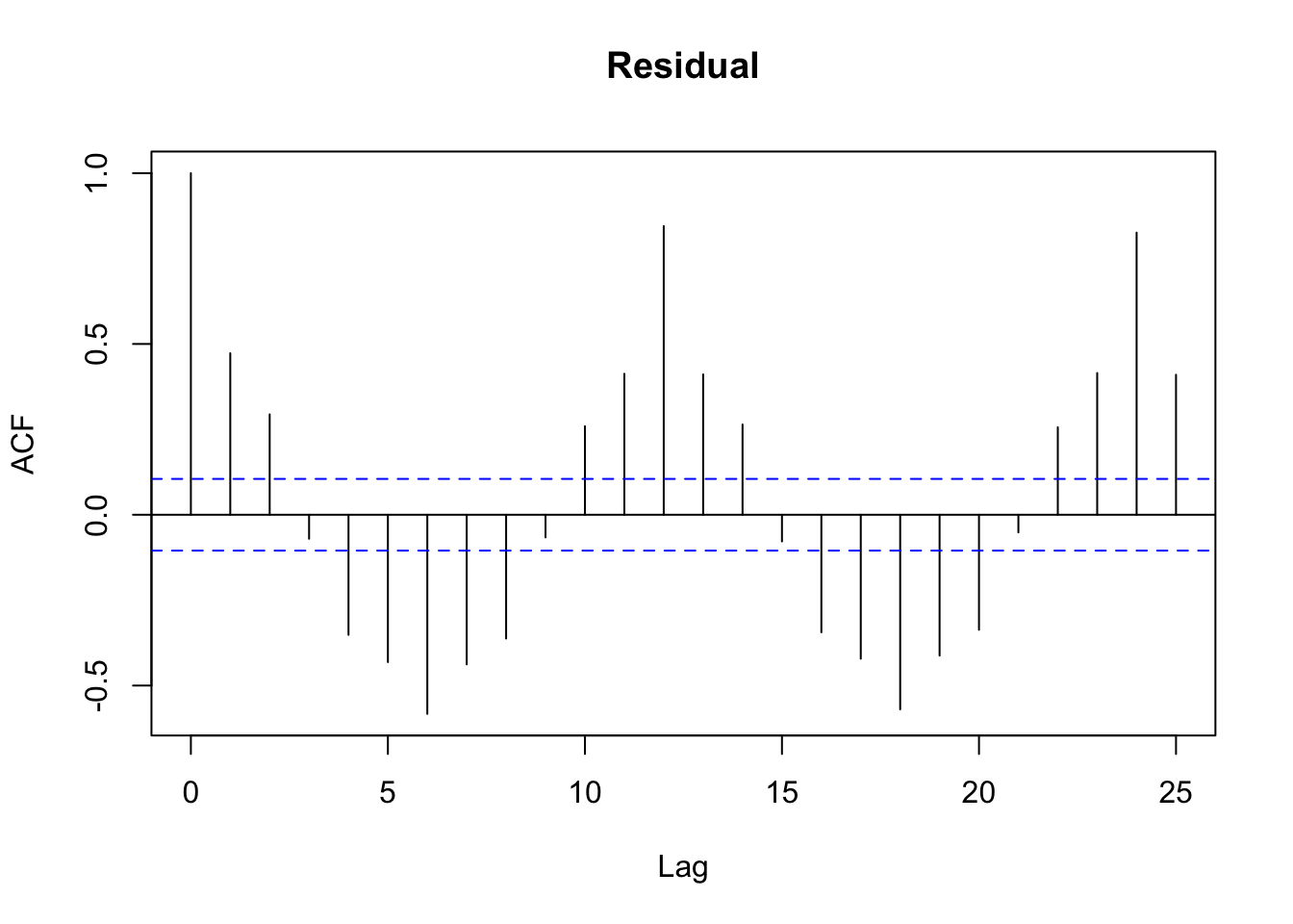
The autocorrelation has to be 1 for lag 0 because \(r_0 = c_0/c_0 = 1\). Note that the lags are in terms of months here because we did not specify a ts() object. We see the autocorrelation slowly decreasing to zero.
What about the ACF of birth data after differencing?
acf(diff(birth, 1)) # one difference to remove trend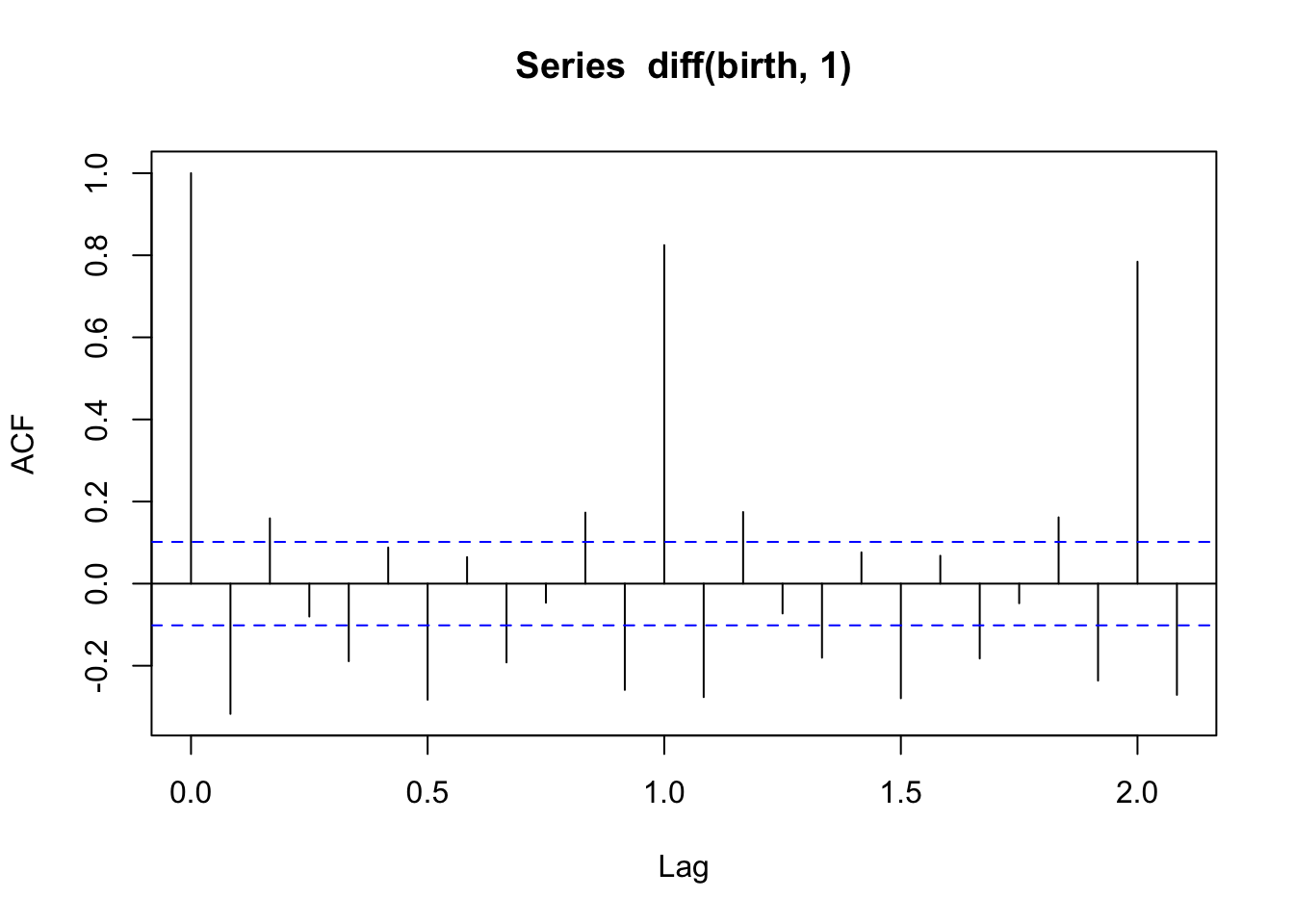
acf(diff(diff(birth,1), lag = 12, 1)) # differences to remove trend and seasonality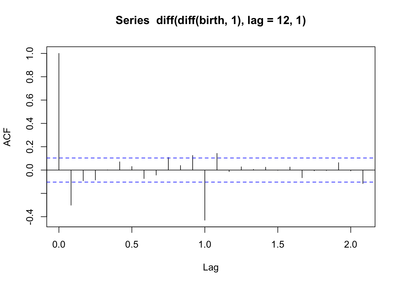
Note that the lags here are in terms of years (Lag = 1 on the plot refers to \(h\) = 12) because the data is saved as a ts object. In the first plot (after only first differencing), we see an autocorrelation of about 0.5 for observations one year apart. This suggests that there may still be some seasonality to be accounted for. In the second plot, after we also did seasonal differencing for lag = 12, that decreases a bit (and becomes a bit negative).
Now, do you notice the blue, dashed horizontal lines?
These blue horizontal lines are guide lines for us. If the random process is white noise such that the observations are independent and identically distributed with a constant mean (of 0) and constant variance \(\sigma^2\), we’d expected the sample autocorrelation to be within these dashed horizontal lines (\(\pm 1.96/\sqrt{n}\)) roughly 95% of the time. So if the random process were independent white noise, we’d expect 95% of the ACF estimates for \(h\not=0\) to be within the blue lines with no systematic pattern.
See an example of Gaussian white noise below and its sample autocorrelation function.
y <- ts(rnorm(500))
plot(y)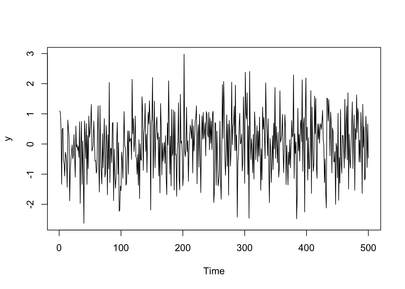
acf(y)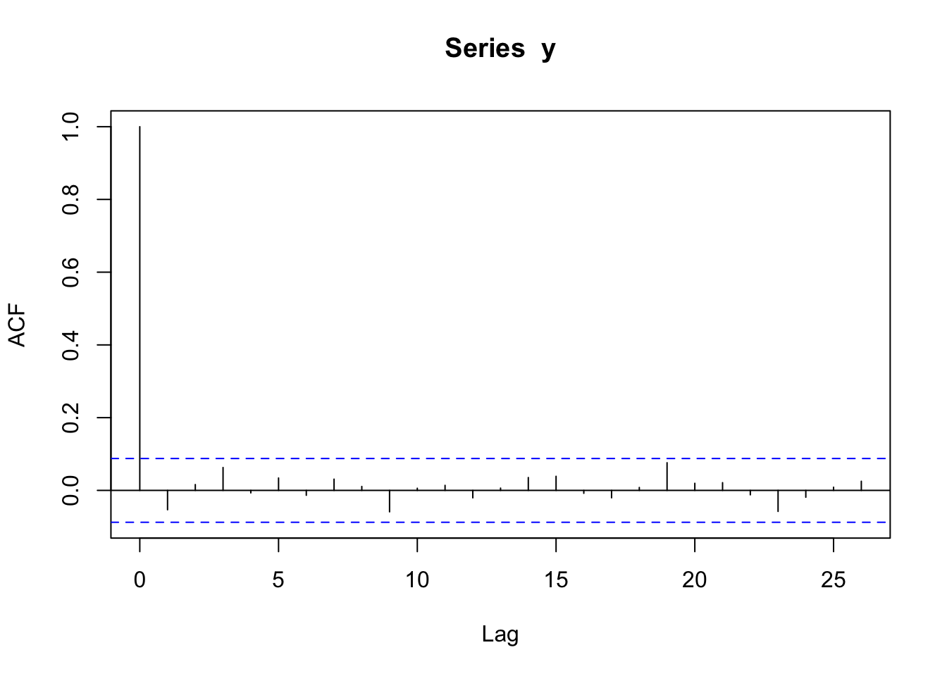
Many stationary time series have recognizable ACF patterns. We’ll get familiar with those in a moment.
However, most time series we encounter in practice are not stationary. Thus, our first step will always be to deal with the trend and seasonality. Then we can model the (hopefully stationary) residuals with a stationary model.
Up to this point, we have decomposed our time series into a trend component, a seasonal component, and a random component,
\[Y_t = \underbrace{f(x_t)}_\text{trend} + \underbrace{s(x_t)}_\text{seasonality} + \underbrace{\epsilon_t}_\text{noise}\]
With observed data, we can work with the residuals after removing the trend and seasonality,
\[e_t = y_t - \underbrace{\hat{f}(x_t)}_\text{trend} - \underbrace{\hat{s}(x_t)}_\text{seasonality} \] which is approximately the true error process,
\[\epsilon_t = Y_t - \underbrace{f(x_t)}_\text{trend} - \underbrace{s(x_t)}_\text{seasonality}\]
For the following time series models (AR, MA, and ARMA), we will use \(Y_t\) to represent the random variable for the residuals, \(e_t\).
In the next five sections, we’ll discuss the theory of these three models. To see a real data example and the R code to fit the models, go to the Real Data Example section.
The first model we will consider for a stationary process is an autoregressive model, which involves regressing current observations on values in the past. So this model regresses on itself (the ‘auto’ part of ‘autoregressive’).
One simple model for correlated errors is an autoregressive order 1 or AR(1) model. The model is stated
\[Y_t = \delta + \phi_1Y_{t-1} + W_t\] where \(W_t \stackrel{iid}{\sim} N(0,\sigma^2_w)\) is independent Gaussian white noise with mean 0 and constant variance, \(\sigma^2_w\). This model is weakly stationary if \(|\phi_1| < 1\).
Note: We will often think of \(\delta = 0\) because our error process is often on average 0.
Properties
Under this model, the expected value (mean) of \(Y_t\) is
\[E(Y_t) = \mu = \frac{\delta}{1-\phi_1}\]
and the variance is
\[Var(Y_t) = \frac{\sigma^2_w}{1-\phi_1^2}\]
The correlation between observations \(h\) lags (time periods) apart is
\[\rho_h = \phi^h_1\]
Derivations for these properties are available in the Appendix at the end of this chapter.
Simulated Data Example
We will generate data from an AR(1) model with \(\phi_1 = 0.64\). For a positive \(\phi_1\), the autocorrelation exponentially decreases to 0 as the lag increases, \(\rho_h = (0.64)^h\).
# Simulate an ar(1) process
# x = 0.05 + 0.64*x(t-1) + e
# Create the vector x
x   <- vector(length=1000)

#simulate the white noise errors
e   <- rnorm(1000)

#Set the coefficient
beta    <- 0.64

# set an initial value
x[1]    <- 0.055

 #Fill the vector x
 for(i in 2:length(x))
    {
        x[i]    <- 0.05 + beta*x[i-1] + e[i]
 }
x <- ts(x)
plot(x)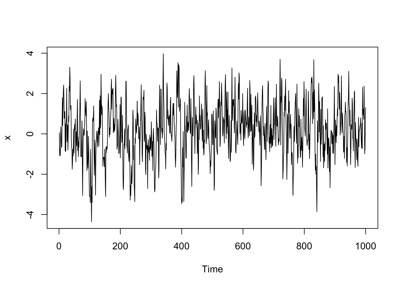
acf(x)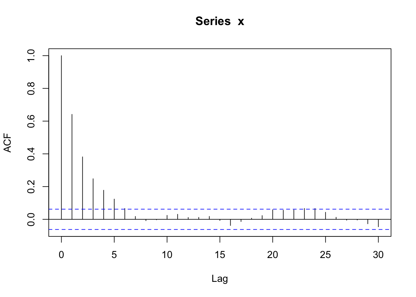
Now, we’ll try \(\phi_1 = -0.8\). For a negative \(\phi_1\), the autocorrelation exponentially decreases to 0 as the lag increases, but the signs of the autocorrelation alternate between positive and negative (\(\rho_h = (-0.8)^h\)).
# Simulate an ar(1) process
# x = 0.05 - 0.8*x(t-1) + e
# Create the vector x
x   <- vector(length=1000)

#simulate the white noise errors
e   <- rnorm(1000)

#Set the coefficient
beta    <- -0.8

# set an initial value
x[1]    <- 0.05

#Fill the vector x
 for(i in 2:length(x))
    {
        x[i]    <- 0.05 + beta*x[i-1] + e[i]
 }
x <- ts(x)
plot(x)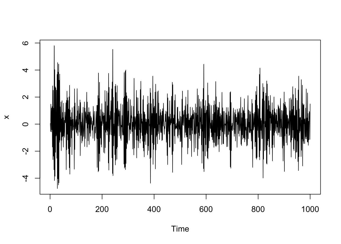
acf(x)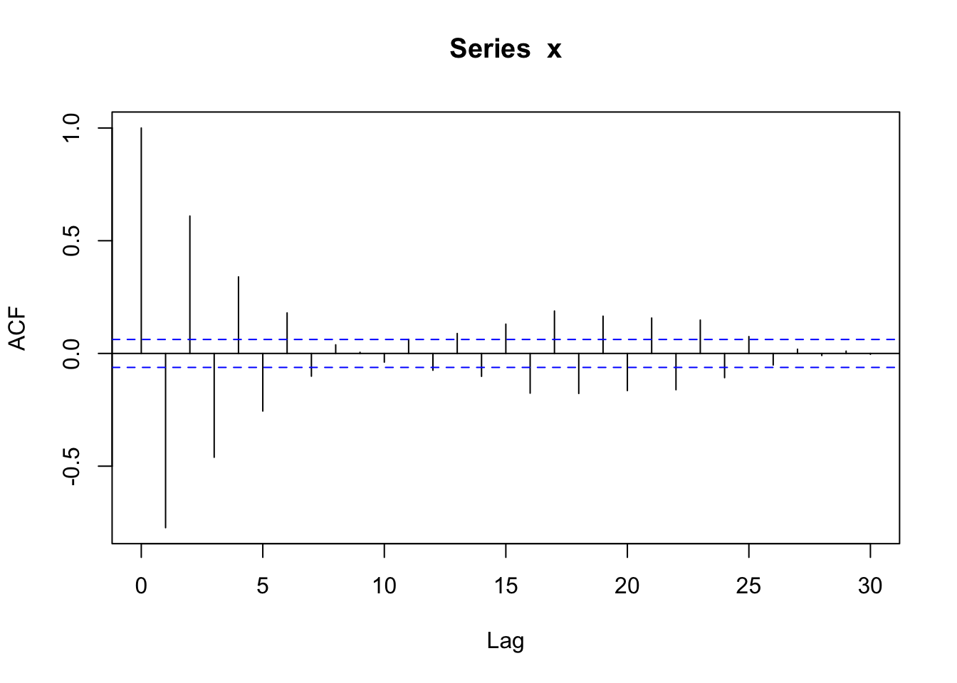
Remember that \(|\phi_1| < 1\) in order for an AR(1) process to be stationary (constant mean, constant variance, autocovariance only depends on lags).
If \(\phi_1 = 1\) and \(\delta = 0\) (a simplifying assumption), the AR(1) model becomes a well-known process called a random walk. The model for a random walk is
\[Y_t = Y_{t-1} + W_t\] where \(W_t \stackrel{iid}{\sim} N(0,\sigma^2_w)\).
If we start with \(t = 1\), then we start with random white noise,
\[Y_1 = W_1\]
The next observation is the past observation plus noise,
\[Y_2 = Y_1 + W_2 = W_1 + W_2\]
The next observation is the past observation plus noise,
\[Y_3 = Y_2 + W_3 = (W_1+W_2)+W_3\]
And so forth,
\[Y_n = Y_{n-1} + W_n = \sum_{i=1}^n W_i\]
So a random walk is the sum of random white noise random variables.
Properties
This random walk process is NOT weakly stationary because the variance is not constant as it is a function of time, \(t\),
\[Var(Y_t) = Var(\sum^t_{i=1} W_i) = \sum^t_{i=1} Var(W_i) = t\sigma^2_w\]
Simulated Data Example
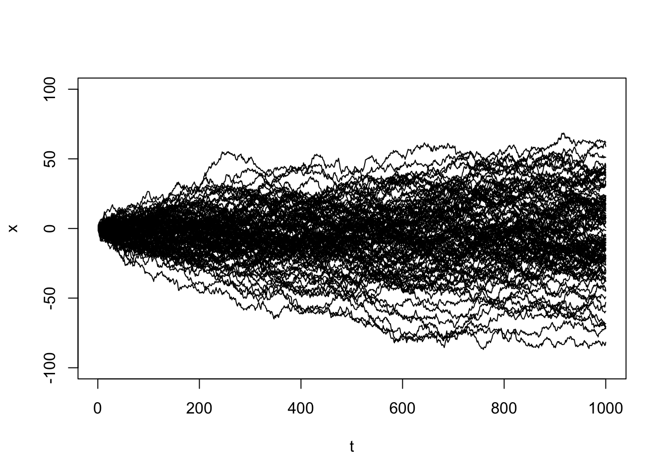
When we generate many random walks, we’ll notice greater potential variability in values later in time. Additionally, you’ll see high autocorrelation at higher lags, indicating a high range of dependence. Two observations that are far in observation time are still highly correlated.
# Simulate one random walk process
# x = x(t-1) + e

#simulate the white noise errors
e   <- rnorm(1000)

# cumulative sum based on recursive process above
x <- cumsum(e)

x <- ts(x)
plot(x)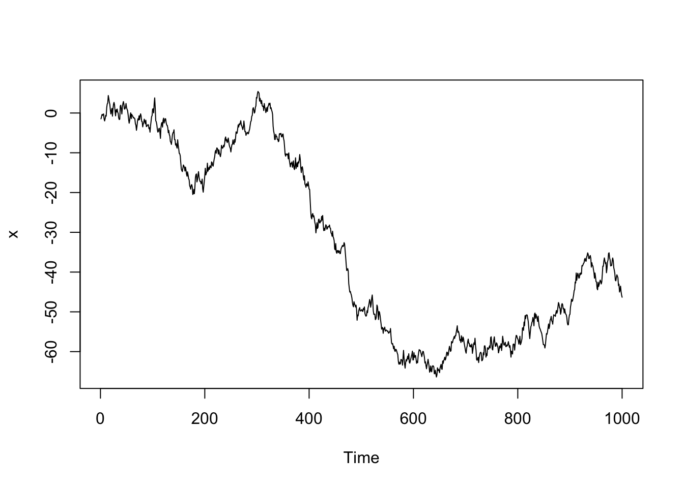
acf(x)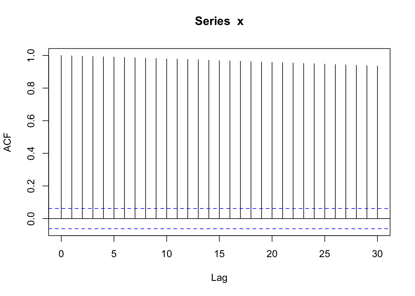
# Simulate many random walk processes
plot(1:1000,rep(1,1000),type='n',ylim=c(-100,100),xlab='t',ylab='x')
for(i in 1:100){
  e <- rnorm(1000)
  x <- cumsum(e)
  x <- ts(x)
  lines(ts(x))
}
If we were to take a first-order difference of a random walk, \(Y_t - Y_{t-1}\), we could remove the trend and end up with independent white noise.
\[Y_t - Y_{t-1}= W_t\]
acf(diff(x, lag = 1, difference = 1))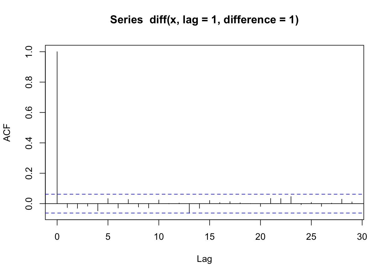
We could generalize the idea of an AR(1) model to allow an observation to be dependent on the past \(p\) previous observations. A autoregression process of order p is modeled as
\[Y_t = \delta + \phi_1Y_{t-1}+ \phi_2Y_{t-2}+\cdots + \phi_pY_{t-p} +W_t\] where \(\{W_t\}\) is independent Gaussian white noise, \(W_t \stackrel{iid}{\sim} N(0,\sigma^2_w)\). We will typically let \(\delta=0\), assuming we have removed the trend and seasonality before applying this model.
Properties
We’ll look at the expected value, variance, and covariance in the AR(p) as MA(\(\infty\)) section after discussing moving average models. We’ll also discuss when the AR(p) model is stationary. I know you can’t wait!
Simulated Data Example
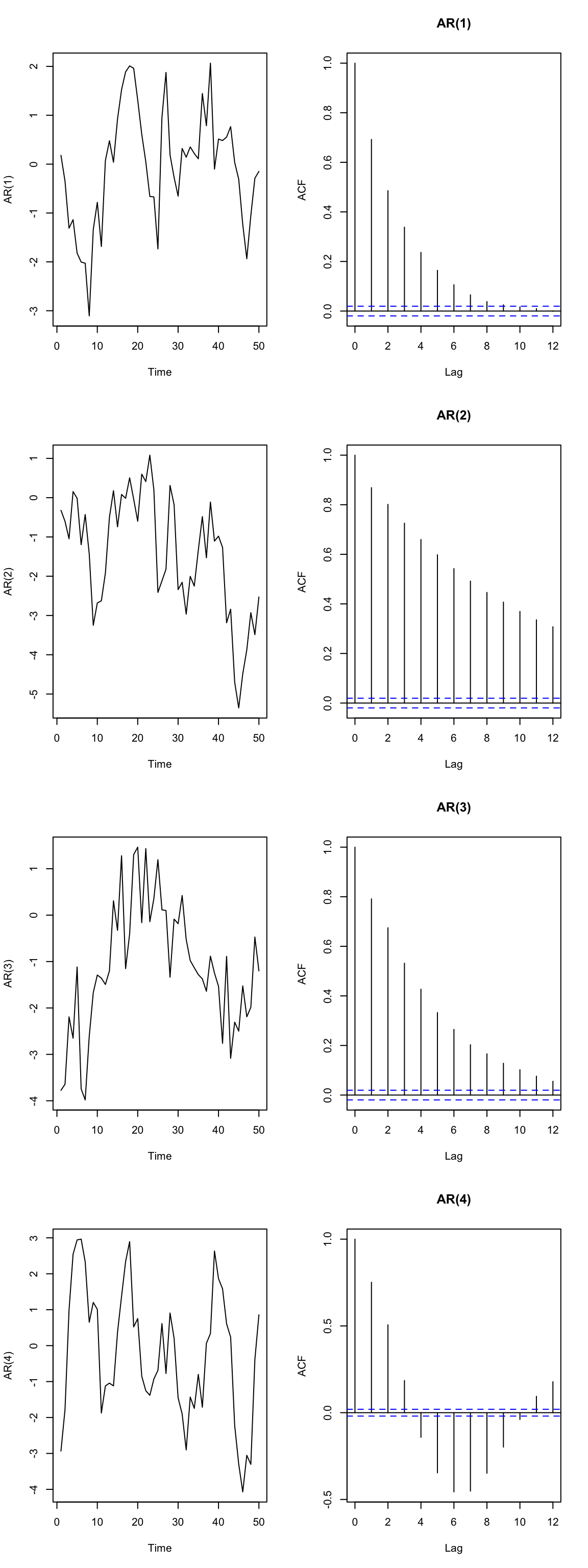
Let’s see a few simulated examples and look at the autocorrelation functions.
set.seed(123)
## the 4 AR coefficients
ARp <- c(0.7, 0.2, -0.1, -0.3)
## empty list for storing models
AR.mods <- list()
## loop over orders of p
for (p in 1:4) {
    ## assume SD=1, so not specified
    AR.mods[[p]] <- arima.sim(n = 10000, list(ar = ARp[1:p]))
}

## set up plot region
par(mfrow = c(4, 2))
## loop over orders of p
for (p in 1:4) {
    plot.ts(AR.mods[[p]][1:50], ylab = paste("AR(", p, ")", sep = ""))
    acf(AR.mods[[p]], lag.max = 12,main=paste("AR(", p, ")", sep = ""))
}
In contrast to the autoregressive model, we will consider a model that considers the current outcome value to be a function of the current and past noise (rather than the past outcomes). This is a subtle difference but you’ll see that a moving average (MA) model is very different than an AR model, but we’ll show how they are connected.
Note: This is different from the moving average filter that we used to estimate the trend.
A moving average process of order 1 or MA(1) model is a weighted sum of a current random error plus the most recent error, and can be written as
\[Y_t = \delta + W_t + \theta_1W_{t-1}\]
where \(\{W_t\}\) is independent Gaussian white noise, \(W_t \stackrel{iid}{\sim} N(0,\sigma^2_w)\).
Like AR models, we often let \(\delta = 0\).
Properties
Unlike AR(1) processes, MA(1) processes are always weakly stationary. We see the variance is constant (not a function of time),
\[Var(Y_t) = Var(W_t + \theta_1W_{t-1}) = \sigma^2_w (1 + \theta_1^2)\]
Let’s look at the autocorrelation function of an MA(1) process.
To derive the autocorrelation function, let’s start with the covariance at lag 1. Plug in the model for \(Y_t\) and \(Y_{t-1}\) and use the properties to simplify the expression,
\[\Sigma_Y(1) = Cov(Y_t, Y_{t-1}) = Cov(W_t + \theta_1W_{t-1}, W_{t-1} + \theta_1W_{t-2})\] \[= Cov(W_t,W_{t-1}) + Cov(W_t, \theta_1W_{t-2}) + Cov(\theta_1W_{t-1}, W_{t-1}) + Cov(\theta_1W_{t-1},\theta_1W_{t-2})\] \[ = 0 + 0 + \theta_1Cov(W_{t-1}, W_{t-1}) + 0\] \[= \theta_1Var(W_{t-1}) \] \[ = \theta_1Var(W_{t}) = \theta_1\sigma^2_w\]
because \(W_t\)’s are independent of each other.
For larger lags \(k>1\),
\[\Sigma_Y(k) = Cov(Y_t, Y_{t-k}) = Cov(W_t + \theta_1W_{t-1}, W_{t-k} + \theta_1W_{t-k-1}) \] \[= Cov(W_t,W_{t-k}) + Cov(W_t, \theta_1W_{t-k-1}) + Cov(\theta_1W_{t-1}, W_{t-k}) + Cov(\theta_1W_{t-1},\theta_1W_{t-k-1})\]
\[ = 0\text{ if }k>1\] because \(W_t\)’s are independent of each other.
Now, the correlation is derived as a function of the covariance divided by the variance (which we found above),
\[\rho_1 = \frac{Cov(Y_t,Y_{t-1})}{Var(Y_t)} = \frac{\Sigma_Y(1)}{Var(Y_t)} = \frac{\theta_1\sigma^2_w}{\sigma^2_w(1+\theta_1^2)} = \frac{\theta_1}{(1+\theta_1^2)}\] and
\[\rho_k = \frac{Cov(Y_t,Y_{t-k})}{Var(Y_t)} = \frac{\Sigma_Y(k)}{Var(Y_t)} = 0\text{ if } k>1\]
So the autocorrelation function is non-zero at lag 1 for an MA(1) process and zero otherwise. Keep this in mind as we look at sample ACF functions.
Simulated Data Example
# Simulate a MA1 process
# x = e + theta1 e(t-1)
# Create the vector x
x   <- vector(length=1000)
theta1 <- 0.5

#simulate the white noise errors
e   <- rnorm(1000)

x[1] <- e[1]

#Fill the vector x
 for(i in 2:length(x))
    {
        x[i]    <- e[i] + theta1*e[i-1]
 }

x <- ts(x)
plot(x)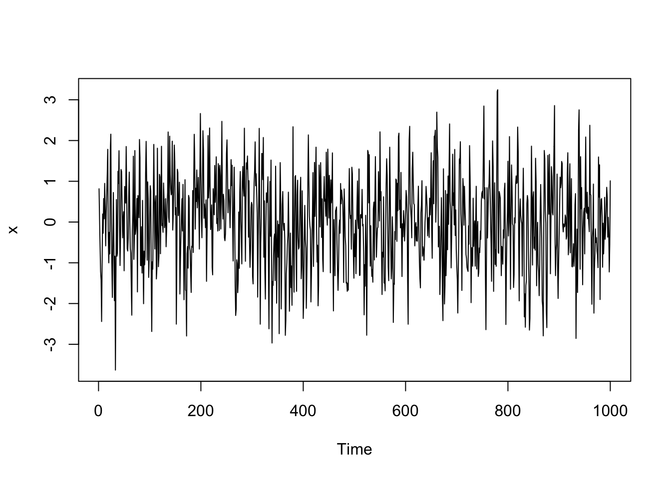
acf(x)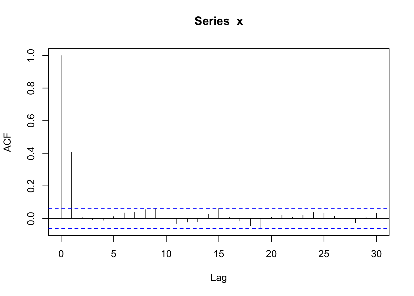
Notice how the autocorrelation = 1 at lag 0 and then around 0.4 at lag 1. The autocorrelation estimate is in between the blue lines for the other lags, so they are practically zero.
Invertibility
No restrictions on \(\theta_1\) are needed for an MA(1) process to be stationary. However, imposing restrictions on \(\theta_1\) is generally desirable to ensure the MA process is invertible.
For an MA process to be invertible, we must be able to write it as an AR(\(\infty\)) process that converges. We’ll talk more about this soon.
We want to restrict ourselves to only invertible processes because of the non-uniqueness of the ACF. Let’s imagine these two processes,
\[A:\quad Y_t = W_t + \theta_1W_{t-1}\] \[B:\quad Y_t = W_t + \frac{1}{\theta_1}W_{t-1}\]
Let’s show that they have the same ACF. We can use our derivations about the MA(1) process. For process B,
\[\rho_1 = \frac{1/\theta_1}{(1+1/\theta_1^2)} = \frac{1}{\theta_1(1+1/\theta_1^2)} = \frac{1}{\theta_1(\frac{\theta_1^2 + 1}{\theta_1^2})}= \frac{1}{\theta_1}\frac{\theta_1^2}{\theta_1^2 + 1} = \frac{\theta_1}{\theta_1^2 + 1}\]
which is the same autocorrelation as process A.
Now, let’s invert process A by rewriting it for \(W_t\) as a function of \(Y_t\),
\[W_t = Y_t - \theta_1W_{t-1}\] and now let’s plug in the model for \(W_{t-1}\),
\[W_t = Y_t - \theta_1(Y_{t-1} - \theta_1W_{t-1}) = Y_t - \theta_1Y_{t-1} - \theta_1^2W_{t-1}\]
and if you keep going, you get an infinite sum,
\[W_t = Y_t - \theta_1(Y_{t-1} - \theta_1W_{t-1}) = Y_t - \theta_1Y_{t-1} - \theta_1^2Y_{t-2} - \cdots\]
or equivalently, an autoregressive model of order \(\infty\) that is stationary if \(|\theta_1| < 1\),
\[Y_t = W_t + \theta_1Y_{t-1} + \theta_1^2Y_{t-2} + \cdots\] Additionally, this infinite sum only converges to a finite value when \(|\theta_1| < 1\).
If you invert the second process (process B), this infinite sum will not converge if \(|\theta_1| < 1\),
\[W_t = Y_t - 1/\theta_1Y_{t-1} - 1/\theta_1^2Y_{t-2} - \cdots\]
Thus, the first process is invertible, and the second is not if \(|\theta_1| < 1\). When we can invert the process, notice that we have written an MA(1) process as an autoregressive process of infinite order.
A moving average process of order q or MA(q) model is a weighted sum of a current random error plus \(q\) most recent errors, and can be written as
\[Y_t = \delta + W_t + \theta_1W_{t-1}+ \theta_2W_{t-2}\cdots + \theta_qW_{t-q}\] where \(\{W_t\}\) is independent Gaussian white noise, \(W_t \stackrel{iid}{\sim} N(0,\sigma^2_w)\). Similar to AR models, we will often let \(\delta=0\).
Properties
As with MA(1), we see the variance is constant (and not a function of time),
\[Var(Y_t) = Var(W_t + \theta_1W_{t-1}+ \theta_2W_{t-2}\cdots + \theta_qW_{t-q}) = \sigma^2_w (1 + \sum^q_{i=1}\theta_i^2)\]
More generally for a MA(q) process, the autocorrelation is non-zero for the first q lags and zero for lags > q.
We can show this for an MA(2) process and higher-order models using the same techniques as before.
Simulated Data Example
# Simulate a MA2 process
# x = e + theta1 e(t-1)  + theta2 e(t-2)
# Create the vector x
x   <- vector(length=1000)
theta1 <- 0.5
theta2 <- -0.2

#simulate the white noise errors
e   <- rnorm(1000)

x[1] <- e[1]
x[2] <- e[2]

#Fill the vector x
 for(i in 3:length(x))
    {
        x[i]    <- e[i] + theta1*e[i-1]  + theta2*e[i-2]
 }

x <- ts(x)
plot(x)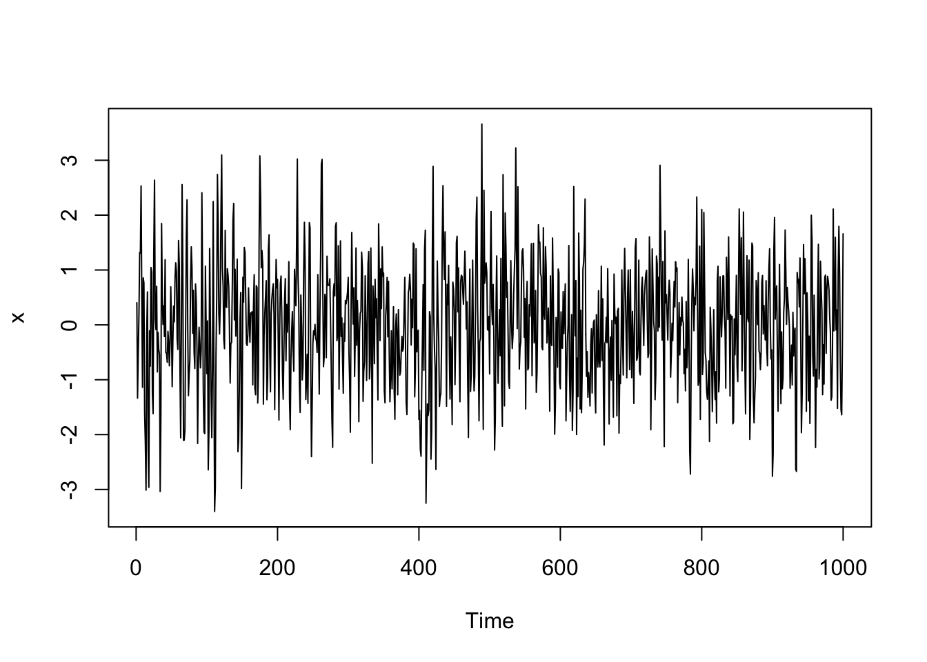
acf(x)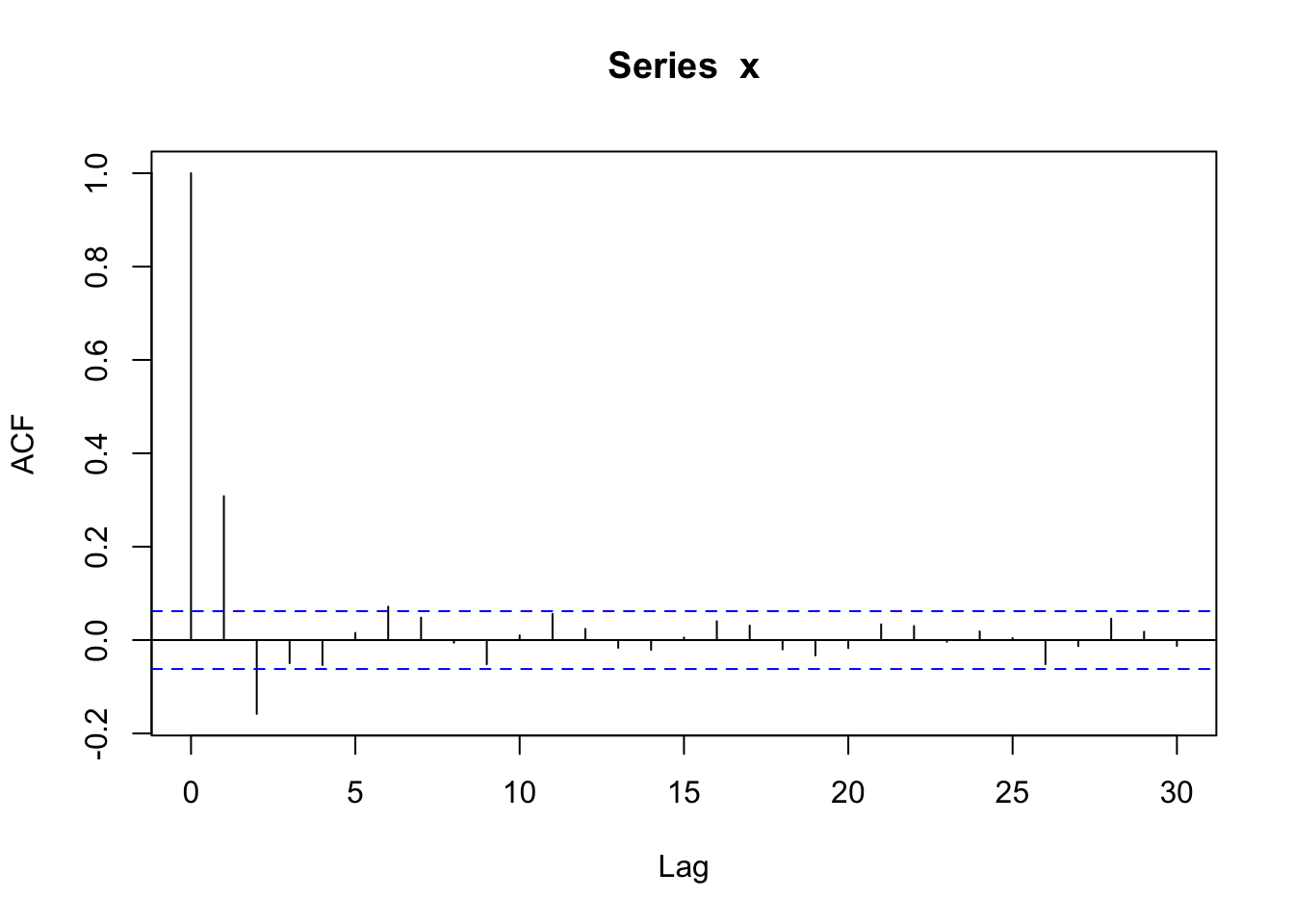
Notice at lag = 0, the autocorrelation is 1, at lag = 1 and 2, the autocorrelation is non-zero for an MA(2) model, and for all other lags, the autocorrelation is practically zero (within blue lines).
Invertibility
To check the invertibility of an MA(q) process, we need to learn about the backward shift operator, denoted \(B\), which is defined as
\[B^jY_t = Y_{t-j}\] The backshift operator is notation that allows us to simplify how we write down the MA(q) model.
The MA(q) model can be written as
\[Y_t = (\theta_0 + \theta_1B + \cdots + \theta_qB^q)W_t \] \[= \theta(B)W_t \]
where \(\theta(B)\) is a polynomial of order \(q\) in terms of \(B\). It can be shown that an MA(q) process is invertible if the roots of the equation,
\(\theta(B) = (\theta_0 + \theta_1B + \cdots + \theta_qB^q) = 0\)
all lie outside the unit circle, where \(B\) is regarded as a complex variable and not an operator.
Remember: the roots are the values of \(B\) in which \(\theta(B) = 0\).
For example, a MA(1) process has a polynomial \(\theta(B) = 1+\theta_1B\) with roots \(B = -1/\theta_1\). This root is a real number, and it is outside the unit circle (\(>|1|\)) as long as \(|\theta_1|<1\). Rarely will you have to check this, but the software we will use restricts the values of \(\theta_j\) so that the process is invertible.
Now, we already see that we can write an MA model as an AR(\(\infty\)) model. Let’s write an AR model as an MA(\(\infty\)) model. This is the main connection between the two models.
Let’s return to an AR(1) model momentarily.
\[Y_t = \phi_1Y_{t-1} + W_t\] By successive substitution, we can rewrite this model is an infinite-order MA model,
\[Y_t = \phi_1(\phi_1Y_{t-2} + W_{t-1}) + W_t =\phi_1^2Y_{t-2} + \phi_1W_{t-1} + W_t \] \[ =\phi_1^2(\phi_1Y_{t-3} + W_{t-2}) + \phi_1W_{t-1} + W_t =\phi_1^3Y_{t-3} + \phi_1^2W_{t-2} + \phi_1W_{t-1} + W_t \] \[ =W_t + \phi_1W_{t-1} +\phi_1^2W_{t-2} +\phi_1^3W_{t-3}+\cdots \] This can also be shown with a backward shift operator,
\[(1-\phi_1 B)Y_t = W_t \implies Y_t = (1-\phi_1 B)^{-1}W_t\] \[Y_t = (1-\phi_1 B)^{-1}W_t\] \[= (1+\phi_1 B + \phi_1^2 B^2 + \cdots )W_t\] This converges when \(|\phi_1|<1\) by the infinite sum rule that \(\sum^\infty_{i=1}r^i = (1-r)^{-1}\) if \(|r|<1\).
With this format, it is clear that for an AR(1) process,
\[E(Y_t) = E(W_t +\phi_1W_{t-1} + \phi_1^2 W_{t-2} + \cdots ) = 0\]
\[Var(Y_t) = Var(W_t +\phi_1W_{t-1} + \phi_1^2 W_{t-2} + \cdots ) = \sigma^2_w(1+\phi_1^2 + \phi_1^4 + \cdots) =\frac{\sigma^2_w}{1-\phi_1^2}\text{ if } |\phi_1|<1\]
A general AR(p) model can be written with a backward shift operator,
\[(1-\phi_1 B-\phi_2 B^2 -\cdots - \phi_p B^p)Y_t = W_t \implies Y_t = (1-\phi_1 B-\phi_2 B^2 -\cdots - \phi_p B^p)^{-1}W_t\]
where \((1-\phi_1 B-\phi_2 B^2 -\cdots - \phi_p B^p)^{-1} = (1 + \beta_1 B + \beta_2B^2 +\cdots)\) (this mathematical statement can be proved, but we won’t get into that in this course). So,
\[Y_t = (1 + \beta_1 B + \beta_2B^2 +\cdots)W_t\]
With this format, it is clear that for an AR(p) process,
\[E(Y_t) = 0\]
\[Var(Y_t) = \sigma^2_w(1+\beta_1^2 + \beta_2^2 + \cdots)\text{ which will be finite if } \sum \beta_i^2\text{ converges}\]
The autocovariance function is given by
\[\Sigma_Y(k) = \sigma^2_w \sum^{\infty}_{i=0}\beta_i \beta_{i+k}\text{ where } \beta_0=1\]
which will converge if \(\sum |\beta_i|\) converges. But, figuring out what the \(\beta_i\)’s should be is hard. There is an easier way to do this.
Let’s go back to the original model statement (but let’s assume \(\delta =0\)),
\[Y_t = \phi_1Y_{t-1}+ \phi_2Y_{t-2}+\cdots + \phi_pY_{t-p} +W_t\]
Multiply that model through by \(Y_{t-k}\),
\[Y_tY_{t-k} = \phi_1Y_{t-1}Y_{t-k}+ \phi_2Y_{t-2}Y_{t-k}+\cdots + \phi_pY_{t-p}Y_{t-k} +W_tY_{t-k}\]
Then take the expectation and divide it by the variance of \(Y_t\), \(Var(Y_t)\) (assuming it is finite)
\[\frac{E(Y_tY_{t-k})}{Var(Y_t)} = \frac{\phi_1E(Y_{t-1}Y_{t-k})}{Var(Y_t)} + \frac{\phi_2E(Y_{t-2}Y_{t-k})}{Var(Y_t)}+ \cdots + \frac{\phi_pE(Y_{t-p}Y_{t-k})}{Var(Y_t)} +\frac{E(W_tY_{t-k})}{Var(Y_t)} \]
Assuming the process is stationary, this simplifies to
\[\rho_k = \phi_1\rho_{k-1}+ \phi_2\rho_{k-2}+ \cdots + \phi_p\rho_{k-p} \text{ for } k = 1,2,...\]
If you plug in estimates of the autocorrelation function for \(k=1,...,p\), and recognize that \(\rho(-k) = \rho(k)\), and solve for these equations, you’ll get the estimates of \(\phi_1,...,\phi_p\). This is a well-posed problem that can be done with matrix notation.
In practice, you will have the computer estimate these models for you. Keep reading for R examples.
You might wonder why it is necessary to know the theoretical properties of the AR and MA models (expected value, variance, covariance, correlation).
This probability theory is important because it will help you choose a model for time series data when you need to choose between the models:
An ARMA(\(p,q\)) model is written as
\[Y_t = \delta + \phi_1Y_{t-1}+ \phi_2Y_{t-2}+\cdots + \phi_pY_{t-p} +W_t +\theta_1W_{t-1}+ \theta_2W_{t-2}\cdots + \theta_qW_{t-q}\] where the white noise \(W_t \stackrel{iid}{\sim} N(0,\sigma^2_w)\).
Equivalently, using the backshift operator, an ARMA model can be written as
\[\phi(B)Y_t = \delta + \theta(B)W_t\] where
\[\phi(B) =1 - \phi_1B- \phi_2B^2 - \cdots - \phi_pB^p\] and
\[\theta(B) = 1+ \theta_1B+ \theta_2B^2 + \cdots + \theta_qB^q\]
In order for the ARMA(\(p\),\(q\)) model
In practice, the computer will restrict the modeling fitting to ARMA weakly stationary and invertible models. But it is important to understand this restriction if you encounter any R errors.
This combined model is useful because you can adequately model a random process with an ARMA model with fewer parameters (\(\phi\)’s or \(\theta\)’s) than a pure AR or pure MA process by itself.
Before we go any further, we need one more tool called the partial autocorrelation function.
The partial autocorrelation function (PACF) measures the linear correlation of an observed value \(\{Y_t\}\) and a lagged version of itself \(\{Y_{t-k}\}\) with the linear dependence of \(\{Y_{t-1},...,Y_{t-(k-1)}\}\) removed. In other words, the PACF is the correlation between two observations in time \(k\) lags apart after accounting for shorter lags.
\[h_k = \begin{cases} \widehat{Cor}(Y_{t},Y_{t-1})\text{ if } k = 1\\ \widehat{Cor}(Y_{t},Y_{t-k} | Y_{t-1},...,Y_{t-(k-1)})\text{ if } k >1 \end{cases}\]
Note that the partial autocorrelation at lag 1 will be the same as the autocorrelation at lag 1. For the other lags, the partial autocorrelation measures the dependence after accounting for the relationships with observations closer in time.
Connection to Stat 155: When we interpret the slope coefficients keeping all other variables fixed, we are interpreting a relationship accounting for those other variables.
Similar to the ACF plots, the dashed horizontal lines indicate plausible values if the random process were independent white noise.
Let’s look at simulated independent Gaussian white noise.
x <- ts(rnorm(1000))
plot(x)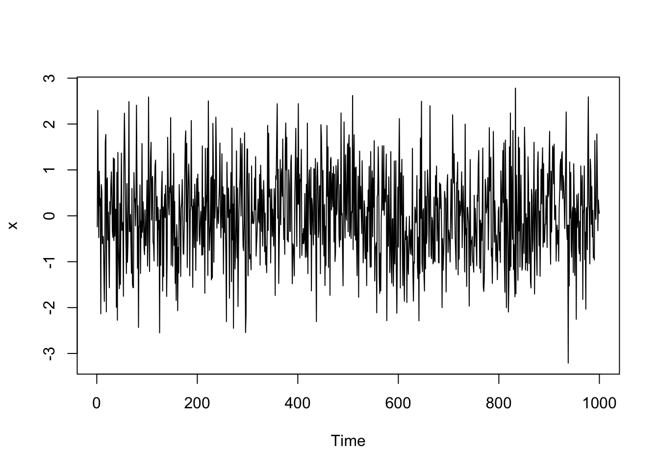
Then, the ACF and the PACF (Partial ACF) functions.
acf2(x)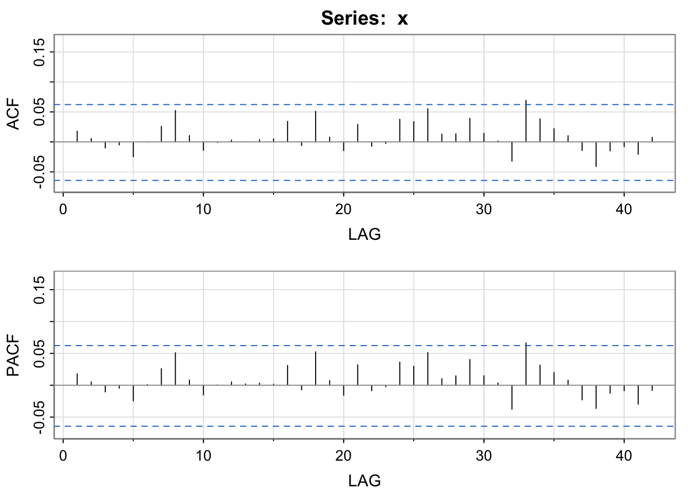
The partial autocorrelation is important to detect the value of \(p\) in an AR(p) model because it has a particular signifying pattern.
For an AR model, the theoretical PACF should be zero past the order of the model. Put another way, the number of non-zero partial autocorrelations gives the order of the AR model, the value of \(p\).
Simulated Data Examples
Let’s see this in action.
Play around with the values of the \(\ phi\)’s and the standard deviation to get a feel for an AR model and its associated ACF and PACF.
x <- arima.sim(n = 1000, list(ar = c(.7, -.3, .5)), sd = 2) #AR(3) model
plot(x)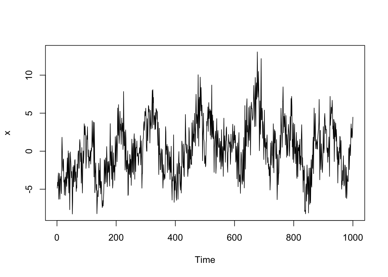
acf2(x)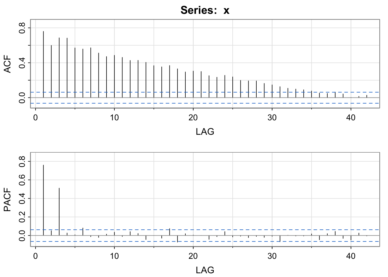
x <- arima.sim(n = 1000, list(ar = c(.8, -.4)), sd = 1) #AR(2) model
plot(x)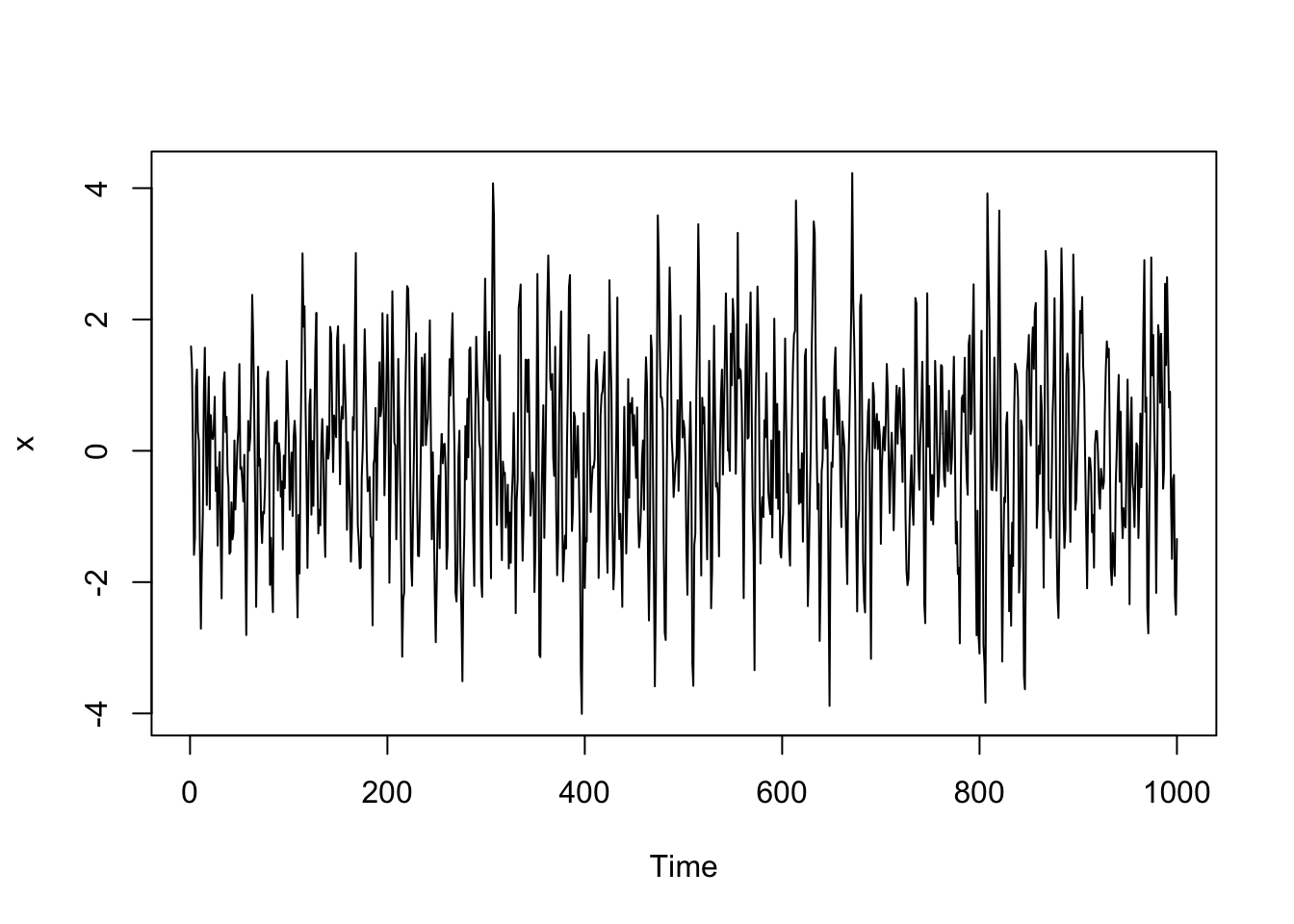
acf2(x)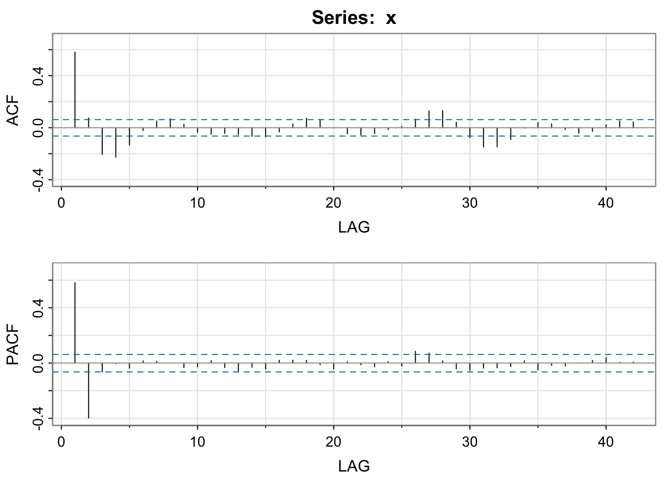
Play around with the values of the \(\theta\)’s and the standard deviation to get a feel for an MA model and its associated ACF and PACF.
x <- arima.sim(n = 1000, list(ma = c(.7, -.2, .8)), sd = 1) #MA(3) model
plot(x)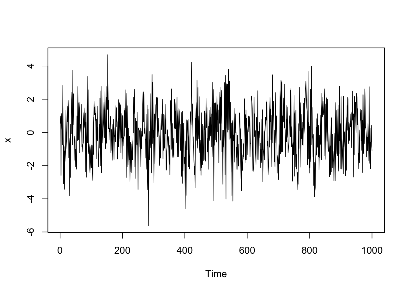
acf2(x)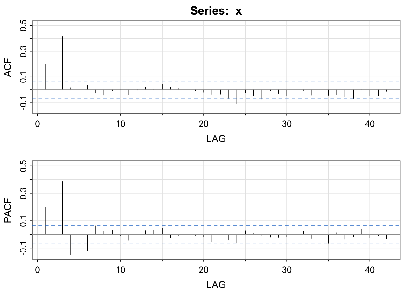
x <- arima.sim(n = 1000, list(ma = c(.8, -.4)), sd = 1) #MA(2) model
plot(x)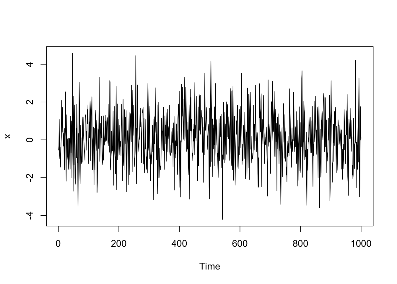
acf2(x)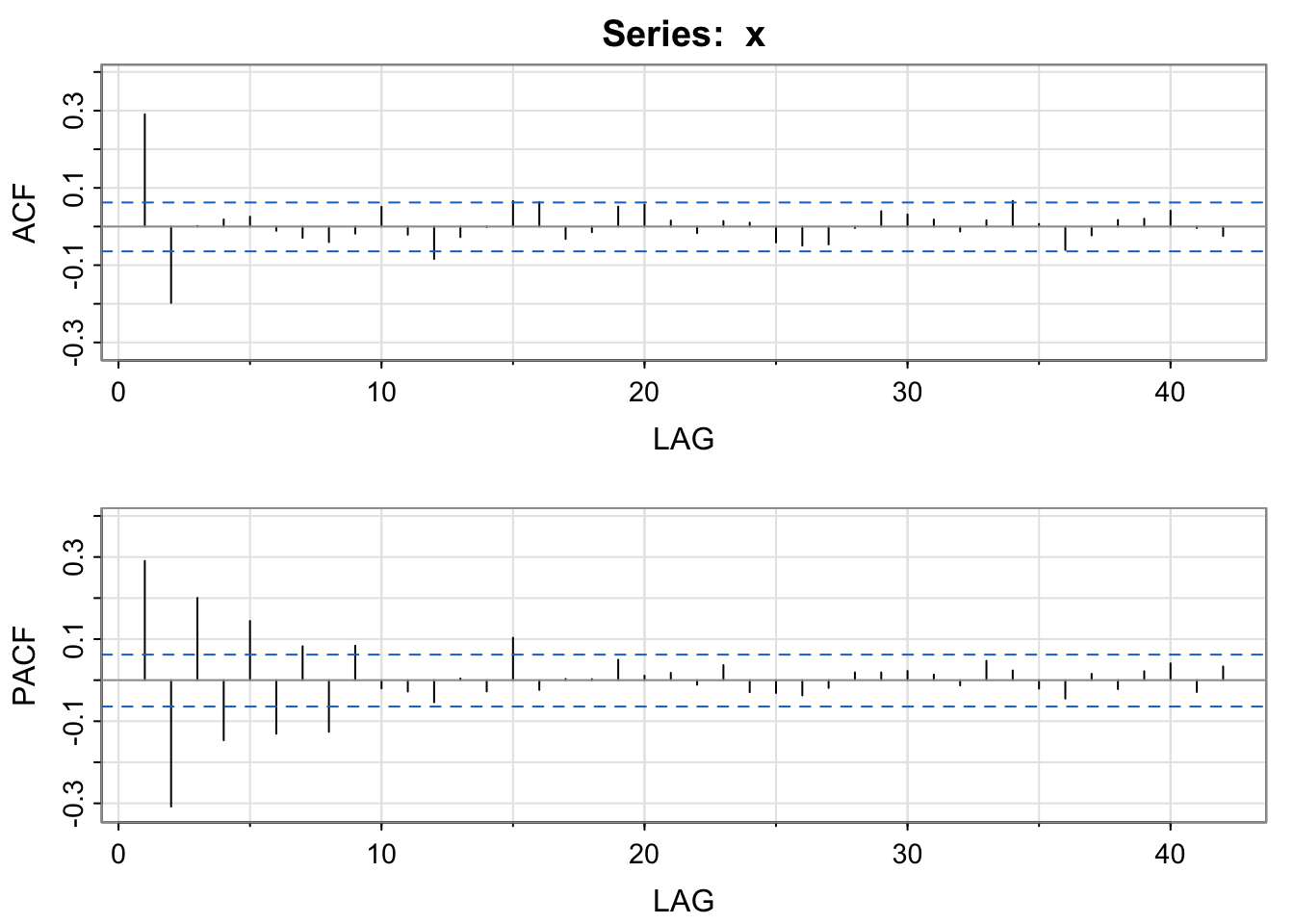
We have now learned about AR(\(p\)), MA(\(q\)), and ARMA(\(p\),\(q\)) models. When we have observed data, we first need to estimate and remove the trend and seasonality and then choose a stationary model to account for the dependence in the errors.
Below, we have a few guidelines and tools to help you work through the modeling process.
Look for possible long-range trends, seasonality of different orders, outliers, constant or non-constant variance.
Model and remove the trend.
Model and remove the seasonality.
Investigate the outliers for possible human errors or find explanations for their extreme values.
If the variability around the trend/seasonality is non-constant, you could transform the series with a logarithm or square root, or use a more complex model such as the ARCH model.
AR(\(p\)) models have PACF non-zero values at lags less than or equal to \(p\) and zero elsewhere. The ACF should decay or taper to zero in some fashion.
MA(\(q\)) models have theoretical ACF with non-zero values at lags less than or equal to \(q\). The PACF should decay or taper to zero in some fashion.
ARMA models (\(p\) and \(q\) > 0) have ACFs and PACFs that taper down to 0. These are the trickiest to determine because the order will not be obvious. Try fitting a model with low orders for one or both \(p\) and \(q\) and compare models.
If the ACF and PACF do not decay to zero but instead have values that stays close to 1 over many lags, the series is non-stationary (non-constant mean) and differencing or estimating to remove the trend will be needed. Try a first difference and look at the ACF and PACF of the difference data.
If all of the autocorrelations are non-significant (within the horizontal lines), then the series is white noise, and you don’t need to model anything. (Great!)
Once we have a potential model that we are considering, we want to make sure that it fits the data well. Below are a few guidelines to check before you determine your final model.
Look at the significance of the coefficients. Are they significantly different from zero? If so, great. If not, they may not be necessary and you should consider changing the order of the model.
Look at the ACF of the residuals. Ideally, our residuals should look like white noise.
Look at a time series plot of the residuals and check for any non-constant variance. If you have non-constant variance in the residuals, consider taking the original data’s natural log and analyzing the log instead of the raw data.
Look at the p-values for the Ljung-Box Test (see Real Data Example for example, R code and output). For this test, \(H_0:\) the data are independent, and \(H_A:\) data exhibit serial correlation (not independent). The test statistic is
\[Q_h = n(n+2)\sum^h_{k=1}\frac{r_k^2}{n-k}\]
where \(h\) is the number of lags being tested simultaneously. If \(H_0\) is true, \(Q_h\) follows a Chi-squared distribution with df = \(h\) for very large \(n\). So you’d like to see large p-values for each lag \(h\) to not reject the \(H_0\).
Which model to choose?
Choose the ‘best’ model with the fewest parameters
Pick the model with the lowest standard errors for predictions in the future
Compare models with respect to the MSE, AIC, and BIC (the lower the better for all)
If two models seem very similar when converted to an infinite order MA, they may be nearly the same. So it may not matter which ARMA model you end up with.
In order to fit these models to real data, we first must get a detrended stationary series (removing seasonality as well). This can be done with estimation and removing, or through differencing.
For the birth data, we tried a variety of ways of removing the trend and seasonality with differencing in the [Model Components] chapter. While the moving average filter worked well. Let’s try a fully parametric approach by using a spline to model the trend and indicators for the seasonality,
library(splines)
birthTS <- data.frame(Year = time(birth), #time() works on ts objects
  Month = cycle(birth), #cycle() works on ts objects
  Value = birth)
birthTS <- birthTS %>%
  mutate(Time = Year + (Month-1)/12)

TrendSeason <- birthTS %>%
  lm(Value ~ bs(Time, degree = 2, knots = c(1965, 1972), Boundary.knots = c(1948,1981)) + factor(Month), data = .)

birthTS <- birthTS %>%
  mutate(ResidualTS = Value - predict(TrendSeason))
The next step is to consider the ACF and PACF to see if you can recognize any clear patterns in dropping or decaying (MA or AR).
acf2(birthTS$ResidualTS) 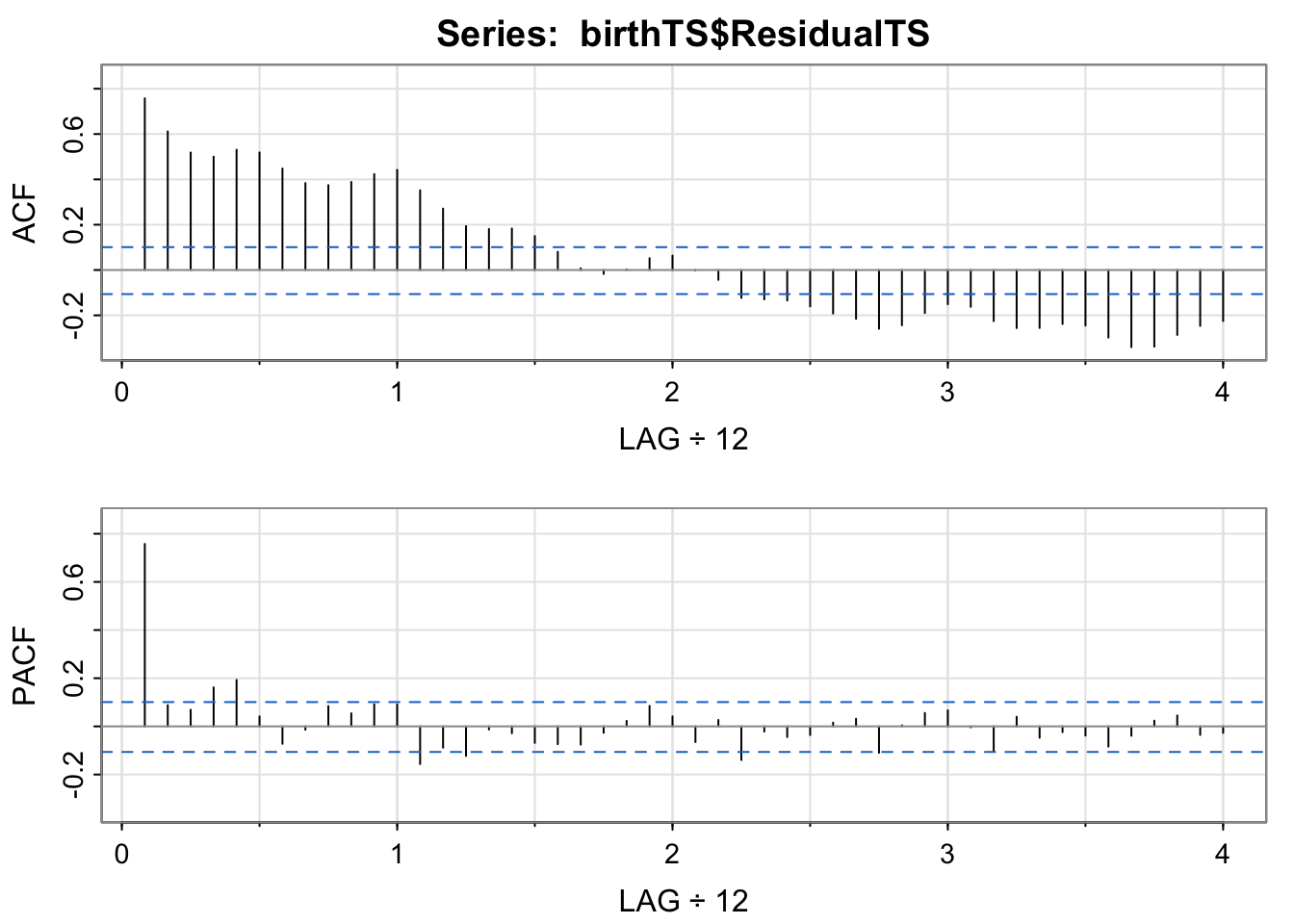
We note the ACF is decaying slowly to zero, and the PACF has 1 clear non-zero lag. These two graphs suggest an AR(1) model. Let’s fit an AR(1) model and a few other candidate models with sarima() in the astsa package.
mod.fit1 <- sarima(birthTS$ResidualTS, p = 1,d = 0,q = 0) #AR(1)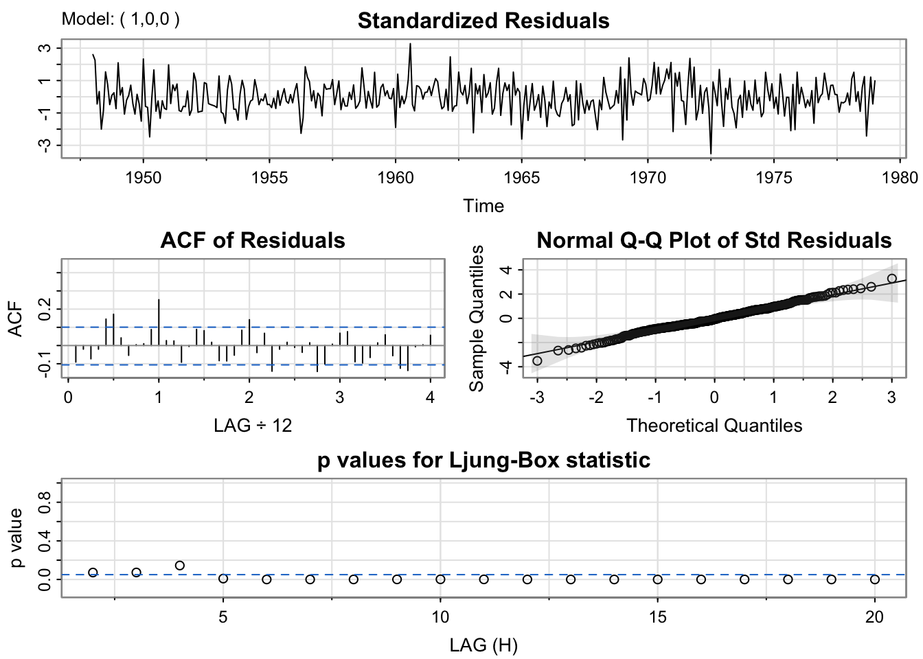
mod.fit1$fit
Call:
arima(x = xdata, order = c(p, d, q), seasonal = list(order = c(P, D, Q), period = S),
    xreg = xmean, include.mean = FALSE, transform.pars = trans, fixed = fixed,
    optim.control = list(trace = trc, REPORT = 1, reltol = tol))

Coefficients:
         ar1   xmean
      0.7709  0.3080
s.e.  0.0334  1.5785

sigma^2 estimated as 49.61:  log likelihood = -1257.84,  aic = 2521.69
mod.fit2 <- sarima(birthTS$ResidualTS, p = 1,d = 0,q = 1) #ARMA(1,1)
mod.fit2$fit
Call:
arima(x = xdata, order = c(p, d, q), seasonal = list(order = c(P, D, Q), period = S),
    xreg = xmean, include.mean = FALSE, transform.pars = trans, fixed = fixed,
    optim.control = list(trace = trc, REPORT = 1, reltol = tol))

Coefficients:
         ar1      ma1   xmean
      0.8557  -0.2106  0.5044
s.e.  0.0412   0.0886  1.9553

sigma^2 estimated as 48.77:  log likelihood = -1254.71,  aic = 2517.41
mod.fit3 <- sarima(birthTS$ResidualTS, p = 2,d = 0,q = 0) #AR(2)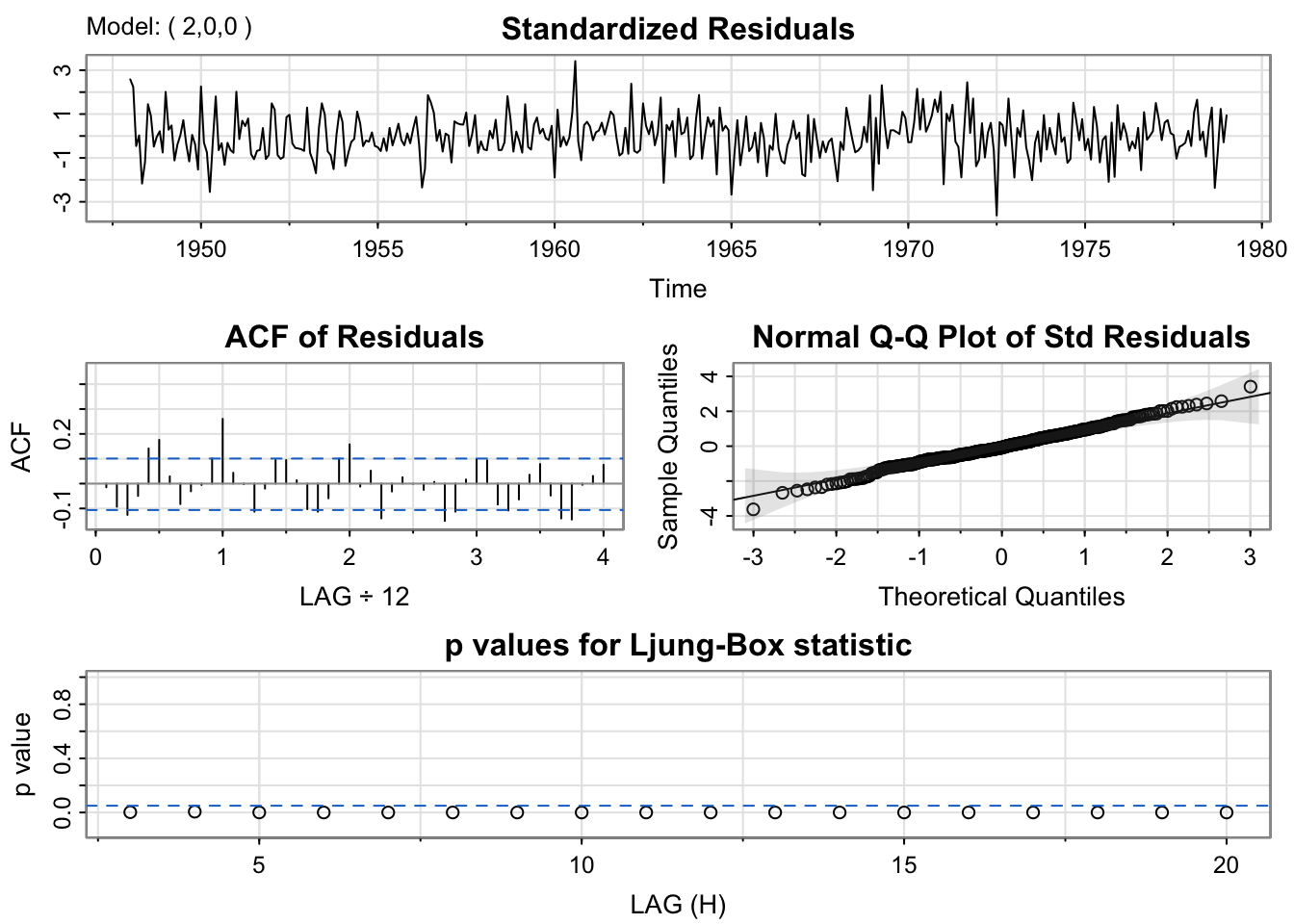
mod.fit3$fit
Call:
arima(x = xdata, order = c(p, d, q), seasonal = list(order = c(P, D, Q), period = S),
    xreg = xmean, include.mean = FALSE, transform.pars = trans, fixed = fixed,
    optim.control = list(trace = trc, REPORT = 1, reltol = tol))

Coefficients:
         ar1     ar2   xmean
      0.6864  0.1127  0.4171
s.e.  0.0514  0.0523  1.7847

sigma^2 estimated as 48.99:  log likelihood = -1255.54,  aic = 2519.07
#Choose a model with lowest BIC
mod.fit1$ICs AIC AICc BIC
6.760554 6.760641 6.792095 mod.fit2$ICs AIC AICc BIC
6.749101 6.749275 6.791155 mod.fit3$ICs AIC AICc BIC
6.753540 6.753714 6.795594 sarima.for(birthTS$ResidualTS,10, p = 1,d = 0,q = 1) #forecasts the residuals 10 time units in the future for the ARMA(1,1) model (we'll get to forecasting in a second)
$pred
          Feb      Mar      Apr      May      Jun      Jul      Aug      Sep
1979 3.505241 3.072234 2.701709 2.384649 2.113339 1.881179 1.682518 1.512523
          Oct      Nov
1979 1.367058 1.242583

$se
           Feb       Mar       Apr       May       Jun       Jul       Aug
1979  6.983803  8.310959  9.161616  9.737476 10.138415 10.422217 10.625218
           Sep       Oct       Nov
1979 10.771436 10.877254 10.954089
Now, you’ll notice that we went through the following steps:
The forecasts look funny because they are only forecasts for errors. If we have taken a parametric approach to estimate the trend and the seasonality, we can incorporate the modeling and removal process in the sarima() function.
First, we need to create a matrix of the variables for the trend and seasonality. We can easily do that with model.matrix() and remove the intercept column with [,-1]. Then we pass that matrix to sarima() with the xreg= argument. This will be useful for us when we do forcasting.
X <- model.matrix(TrendSeason)[,-1] #remove the intercept

GoodMod <- sarima(birthTS$Value, p = 1,d = 0, q = 1, xreg = X)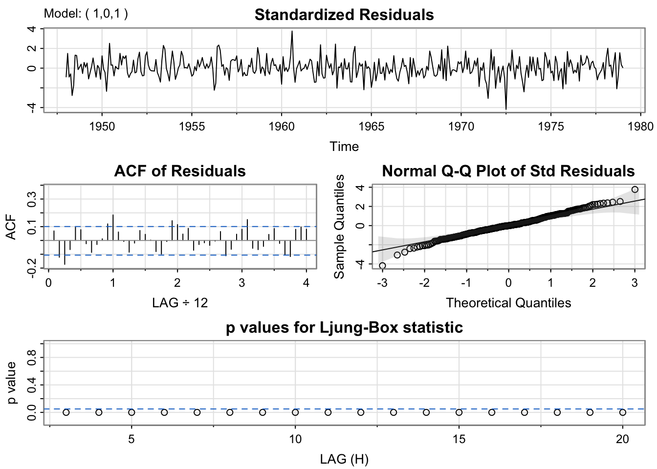
Now, you should notice two things from this output:
There is a slightly higher ACF of residuals at lag 1.0 (at 12 months or 1 year – which is the period of the seasonality)
The p-values for the Ljung-Box statistic are all < 0.05. That is not ideal because it suggests that the residuals of the full model are not independent white noise. There is still dependence that we need to account for with the model.
We’ll come back to fix this. Before we do that, let’s talk about the function being called sarima() instead of arma(). What does the i' stand for, and what does thes` stand for? Read the next section to find out!
ARIMA models are the same as ARMA models, but the i' stands for 'integrated', which refers to differencing. If you were differencing to remove the trend and seasonality, you could incorporate that difference in the model fitting procedure (like we did with the parametric modeling andxreg=`).
Below, we show fitting the model on the ORIGINAL data before removing the trend or seasonality. Then we do a first difference to remove the trend and a first-order difference of lag 12 to remove the seasonality.
The little \(d\) indicates the order of differences for lag 1, the big \(D\) indicates the order of seasonal differences, and \(S\) gives the lag for the seasonal differences. Once we know the differencing that we need to do, we incorporate the differencing into the model fitting, which will give us more accurate predictions for the future.
mod.fit4 <- sarima(birth, p = 0, d = 1, q = 1, D = 1, S = 12) #this model includes lag 1 differencing and lag 12 differencing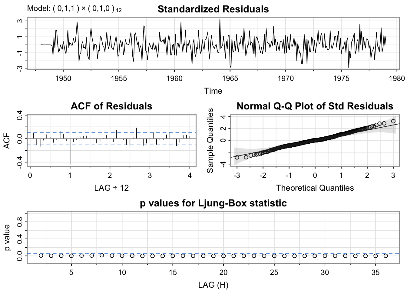
mod.fit4$fit
Call:
arima(x = xdata, order = c(p, d, q), seasonal = list(order = c(P, D, Q), period = S),
    include.mean = !no.constant, transform.pars = trans, fixed = fixed, optim.control = list(trace = trc,
        REPORT = 1, reltol = tol))

Coefficients:
          ma1
      -0.5221
s.e.   0.0547

sigma^2 estimated as 71.62:  log likelihood = -1279.83,  aic = 2563.65
Notice, this model with differencing isn’t any better than the ARMA model with the spline trend and indicator variables for the month.
The s in the sarima() is seasonal. A Seasonal ARIMA model allows us to add a seasonal lag (e.g., 12) into an ARMA model. The model is written as
\[\Phi(B^S)\phi(B)Y_t = \Theta(B^S)\theta(B)W_t\] where the non-seasonal components are: \[\phi(B) =1 - \phi_1B- \phi_2B^2 - \cdots - \phi_pB^p\] and \[\theta(B) = 1+ \theta_1B+ \theta_2B^2 + \cdots + \theta_qB^q\] and the seasonal components are: \[\Phi(B^S) =1 - \Phi_1B^S- \Phi_2B^{2S} - \cdots - \Phi_pB^{PS}\] and \[\Theta(B^S) = 1+ \Theta_1B^S+ \Theta_2B^{2S} + \cdots + \Theta_qB^{QS}\]
Why you might need a Seasonal ARMA?
If you see strong seasonal autocorrelation in the residuals after you fit a good ARMA model, try a seasonal ARMA.
If strong seasonal autocorrelation (non-zero values at lag \(S\), \(2S\), etc.) drops off after Q seasonal lags, you can fit a seasonal MA(Q) model.
On the other hand, if you see a strong seasonal partial autocorrelation that drops off after P seasonal lags, you can fit a seasonal AR(P) model.
acf2(resid(GoodMod$fit)) #Notice the high ACF and PACF for lag 1 year (12 months) -- only look at 1 year, 2 years, etc., is there a pattern?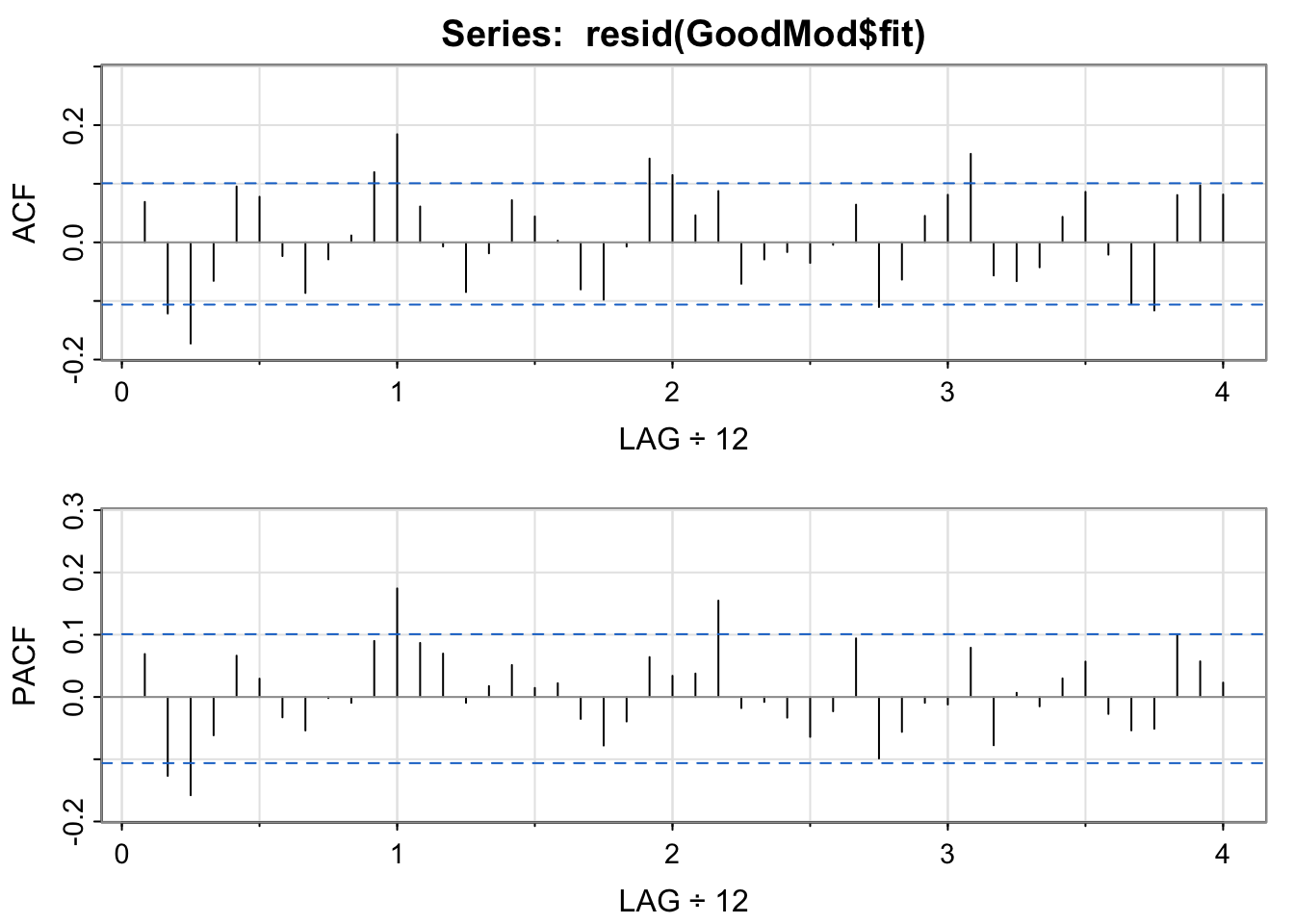
mod.fit5 <- sarima(birthTS$Value, p = 1,d = 0, q = 1,P = 0, D = 0, Q = 1, S = 12, xreg = X) #ARMA(1,1) + SeasonalMA(1)Warning in arima(xdata, order = c(p, d, q), seasonal = list(order = c(P, :
possible convergence problem: optim gave code = 1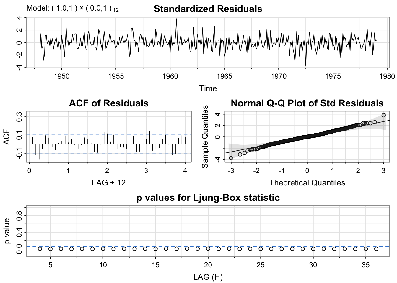
mod.fit6 <- sarima(birthTS$Value, p = 1,d = 0, q = 1,P = 1, D = 0, Q = 0, S = 12, xreg = X) #ARMA(1,1) + SeasonalAR(1)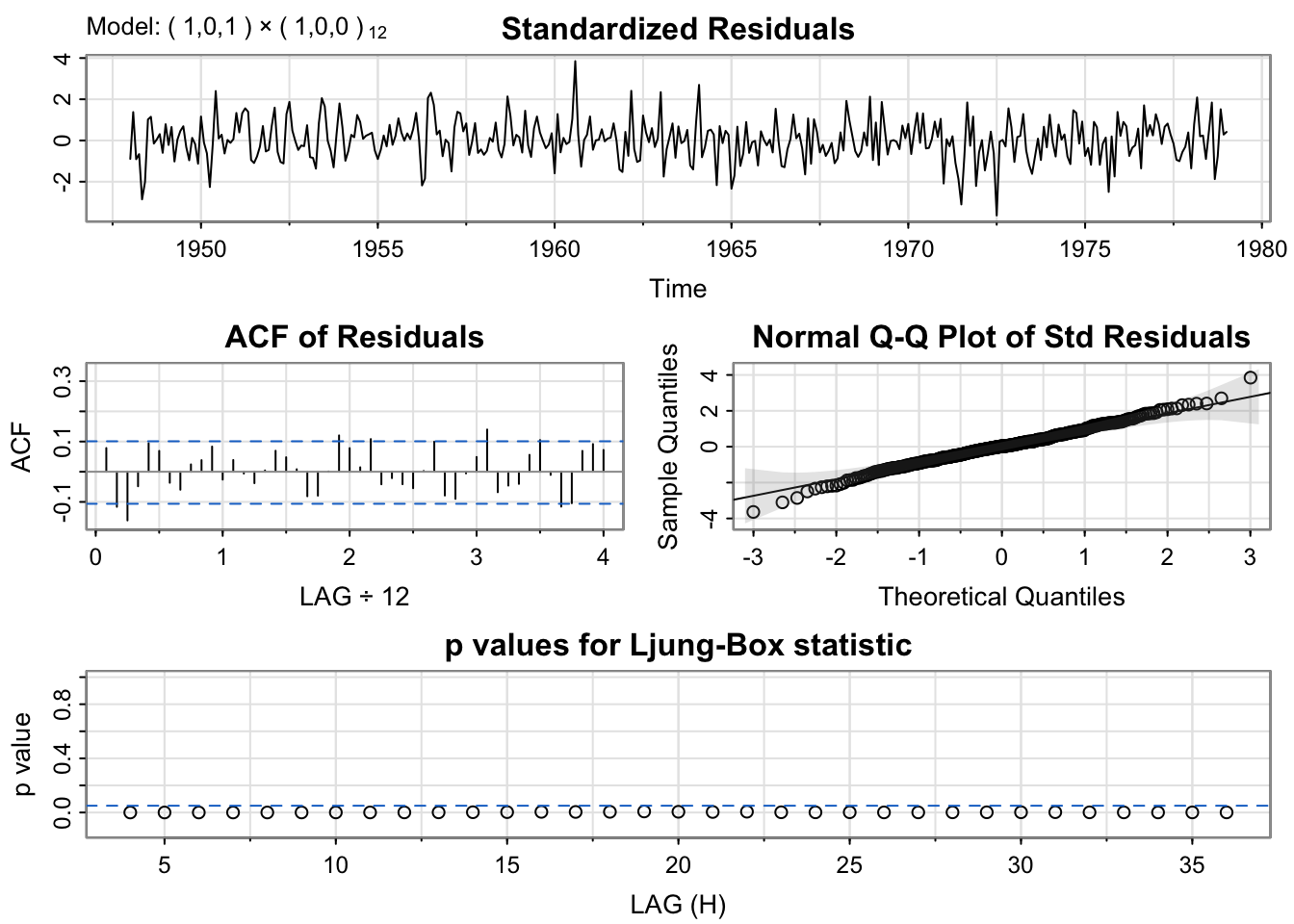
GoodMod$ICs AIC AICc BIC
6.763844 6.769024 6.963603 mod.fit6$ICs AIC AICc BIC
6.728734 6.734506 6.939007 mod.fit5$ICs AIC AICc BIC
6.736525 6.742298 6.946798 While the p-values are still not ideal, the model with spline trend, indicator variables for the month, ARMA(1,1) + SeasonalAR(1) for errors has the lowest BIC, and the SARIMA coefficients are all significantly different from zero.
Typically, when we are working with time series, we want to make predictions for the near future based on recently observed data.
Let’s think about an example. Imagine we had data \(y_1,...,y_n\) and we estimated the mean and seasonality such that \(e_t = y_t - \underbrace{\hat{f}(t|y_1,...,y_n)}_\text{trend} - \underbrace{\hat{S}(t|y_1,...,y_n)}_\text{seasonality}\). Thus, if we knew or had a prediction of \(e_t\), we could get a prediction of \(y_t = \underbrace{\hat{f}(t|y_1,...,y_n)}_\text{trend} + \underbrace{\hat{S}(t|y_1,...,y_n)}_\text{seasonality} + e_t\).
Let’s say we modeled \(e_t\) with an AR(2) process, then
\[e_t = \phi_1e_{t-1} + \phi_2e_{t-2} + W_t\quad\quad W_t\stackrel{iid}{\sim} N(0,\sigma^2_w)\]
Since we have data for \(y_1,...,y_n\), we have data for \(e_1,...,e_n\) to use to estimate \(\phi_1\), \(\phi_2\), and \(\sigma^2_w\).
To get a one-step ahead prediction based on the \(n\) observed data points, \(e_{n+1}^n\), we could plug into our model equation,
\[e_{n+1} = \phi_1e_{n} + \phi_2e_{n-1} + W_{n+1}\quad\quad W_t\stackrel{iid}{\sim} N(0,\sigma^2_w)\] We do have the values of \(e_n\) and \(e_{n-1}\) plus estimates of \(\phi_1\) and \(\phi_2\). But we don’t know \(w_{n+1}\). However, we know that our white noise is about 0 on average. So, our prediction one step ahead based on \(n\) observed data points is
\[\hat{e}^n_{n+1} = \hat{\phi_1}e_{n} + \hat{\phi_2}e_{n-1}\]
What about two steps ahead? If we plug it into our model,
\[e_{n+2} = \phi_1e_{n+1} + \phi_2e_{n} + W_{n+2}\quad\quad W_t\stackrel{iid}{\sim} N(0,\sigma^2_w)\]
we see that we do have the value of \(e_n\) plus estimates of \(\phi_1\) and \(\phi_2\). But we don’t know \(e_{n+1}\) and \(W_{n+2}\). Similar to before, we can assume the white noise is, on average, 0, and we can plug in our predictions. So, our two-step ahead prediction based on \(n\) data points is
\[\hat{e}^n_{n+2} = \hat{\phi_1}\hat{e}_{n+1}^n + \hat{\phi_2}e_{n}\]
We could continue this process,
\[\hat{e}^n_{n+m} = \hat{\phi_1}\hat{e}_{n+m-1}^n + \hat{\phi_2}\hat{e}_{n+m-2}^n\]
for \(m>2\). In general, to do forecasting with an ARMA model, for \(1\leq j\leq n\) we use residuals for \(w_j\) and let \(w_j = 0\) for \(j>n\). Similarly, for \(1\leq j\leq n\), we use observed data for \(e_j\) and plug in the forecasts \(\hat{e}_j^n\) for \(j>n\).
We know that our predictions will be off from the truth. But how far off?
Before we can estimate the standard deviation of our errors, we need to know one more thing about ARMA models.
With a stationary ARMA model, we can write it as an infinite MA process (similar to the AR to infinite MA process),
\[Y_t = \sum^\infty_{j=0} \Psi_j W_{t-j}\]
where \(\Psi_0 = 1\) and \(\sum^\infty_{j=1}|\Psi_j|<\infty\).
The R command ARMAtoMA(ar = 0.6, ma = 0, 12) gives the first 12 values of \(\Psi_j\) for an AR(1) model with \(\phi_1 = 0.6\).
ARMAtoMA(ar = 0.6, ma = 0, 12) [1] 0.600000000 0.360000000 0.216000000 0.129600000 0.077760000 0.046656000
[7] 0.027993600 0.016796160 0.010077696 0.006046618 0.003627971 0.002176782The R command ARMAtoMA(ar = 0.6, ma = 0.1, 12) gives the first 12 values of \(\Psi_j\) for an ARMA(1,1) model with \(\phi_1 = 0.6\) and \(\theta_1 = 0.1\).
ARMAtoMA(ar = 0.6, ma = 0.1, 12) [1] 0.700000000 0.420000000 0.252000000 0.151200000 0.090720000 0.054432000
[7] 0.032659200 0.019595520 0.011757312 0.007054387 0.004232632 0.002539579In order to create a prediction interval for \(\hat{y}^n_{n+m}\), we need to know how big the error, \(y^n_{n+m}-y_{n+m}\), may be.
It can be shown that
\[Var(\hat{y}^n_{n+m}-y_{n+m}) = \sigma^2_w \sum^{m-1}_{j=0} \Psi^2_j\] and thus, the standard errors are
\[SE(\hat{y}^n_{n+m}-y_{n+m}) = \sqrt{\hat{\sigma}^2_w \sum^{m-1}_{j=0} \hat{\Psi}^2_j}\]
where \(\hat{\sigma^2_w}\) and \(\hat{\Psi}_j\) are given by the estimation process.
Let’s see this play out with our birth data. We can estimate the ARMA model with sarima() and pull out the estimates of the sigma and the \(\ Psi_j\)’s. Compare our hand calculations to the standard errors from arima.for().
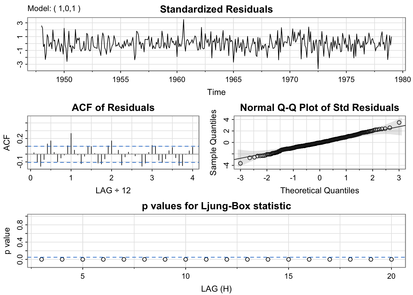
sarima(birthTS$ResidualTS, p = 1,0,q = 1)initial value 2.384529
iter 2 value 2.179452
iter 3 value 2.052027
iter 4 value 2.026011
iter 5 value 1.962581
iter 6 value 1.952577
iter 7 value 1.935739
iter 8 value 1.934205
iter 9 value 1.933599
iter 10 value 1.933531
iter 11 value 1.933495
iter 12 value 1.933483
iter 13 value 1.933478
iter 14 value 1.933470
iter 15 value 1.933456
iter 16 value 1.933451
iter 17 value 1.933448
iter 18 value 1.933444
iter 19 value 1.933443
iter 20 value 1.933440
iter 21 value 1.933436
iter 22 value 1.933433
iter 23 value 1.933433
iter 24 value 1.933433
iter 25 value 1.933433
iter 25 value 1.933433
iter 25 value 1.933433
final value 1.933433
converged
initial value 1.945918
iter 2 value 1.945242
iter 3 value 1.945221
iter 4 value 1.945011
iter 5 value 1.944980
iter 6 value 1.944962
iter 7 value 1.944938
iter 8 value 1.944909
iter 9 value 1.944900
iter 10 value 1.944897
iter 11 value 1.944892
iter 12 value 1.944889
iter 13 value 1.944888
iter 14 value 1.944888
iter 14 value 1.944888
iter 14 value 1.944888
final value 1.944888
converged
<><><><><><><><><><><><><><>
Coefficients:
Estimate SE t.value p.value
ar1 0.8557 0.0412 20.7562 0.0000
ma1 -0.2106 0.0886 -2.3770 0.0180
xmean 0.5044 1.9553 0.2580 0.7966
sigma^2 estimated as 48.77351 on 370 degrees of freedom
AIC = 6.749101 AICc = 6.749275 BIC = 6.791155
psi = c(1,ARMAtoMA(ar = .8727,ma = -0.2469, 9))
sigma2 = 43.5

sarima.for(birthTS$ResidualTS, n.ahead=10, p = 1, d = 0, q = 1)$se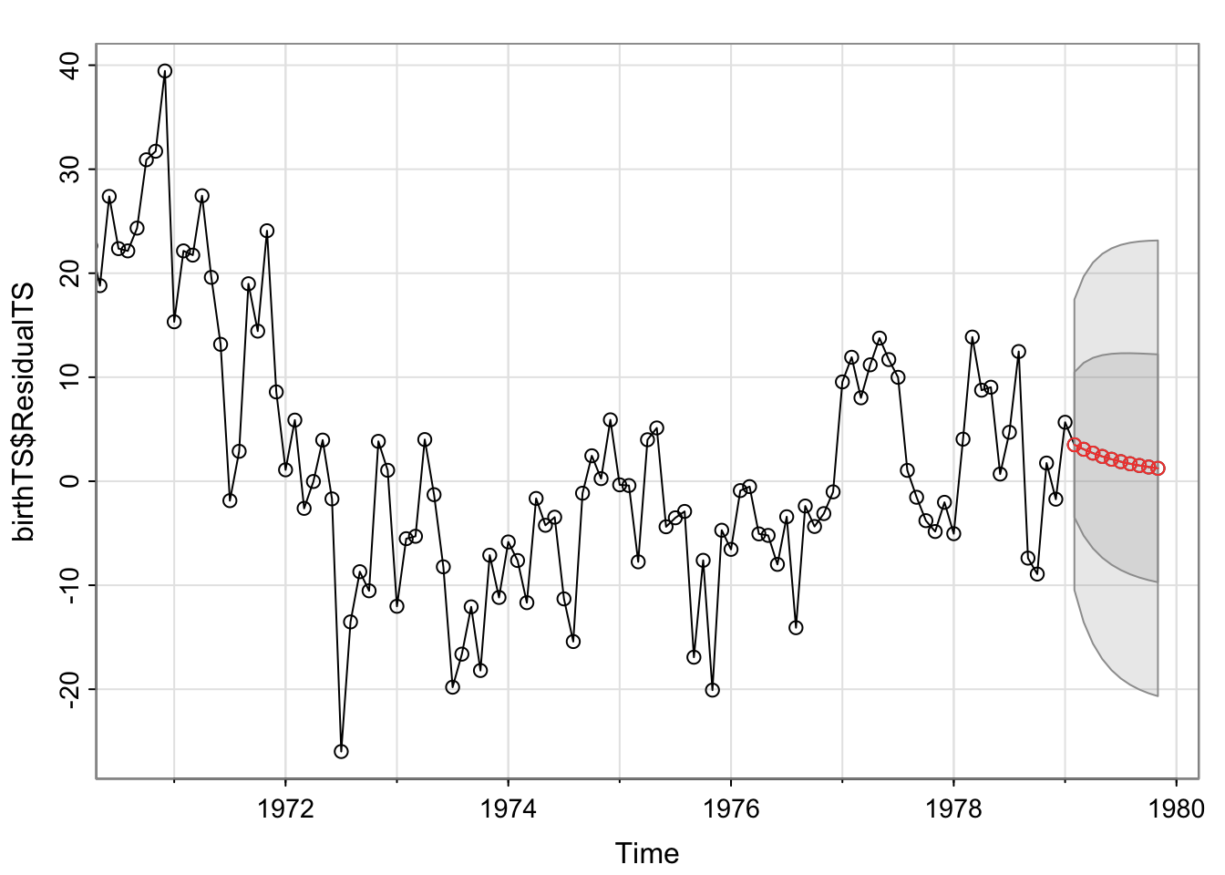
           Feb       Mar       Apr       May       Jun       Jul       Aug
1979  6.983803  8.310959  9.161616  9.737476 10.138415 10.422217 10.625218
           Sep       Oct       Nov
1979 10.771436 10.877254 10.954089sqrt(sigma2*cumsum(psi^2)) #The SE for the predictions are the same [1] 6.595453 7.780470 8.573809 9.131903 9.535062 9.831025 10.050588
[8] 10.214643 10.337841 10.430694But if we incorporate the differencing for the trend/seasonality into the model, we’ll get forecasts in the original units of \(y_t\) instead of just \(Y_t\).
sarima.for(birth, n.ahead = 24, p = 0, d = 1, q = 1, P = 0, D = 1, Q = 1, S = 12)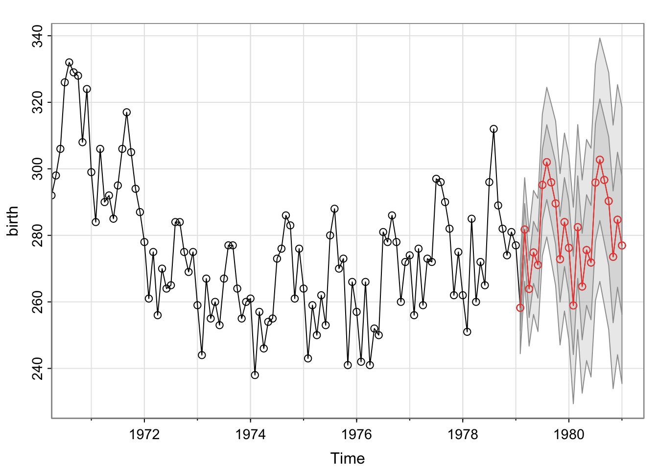
$pred
          Jan      Feb      Mar      Apr      May      Jun      Jul      Aug
1979          258.2172 281.7558 263.9016 274.8702 271.1040 295.1588 302.0120
1980 276.2490 258.9313 282.4699 264.6157 275.5843 271.8181 295.8729 302.7261
1981 276.9632
          Sep      Oct      Nov      Dec
1979 295.9419 289.5935 272.8265 283.9909
1980 296.6561 290.3076 273.5406 284.7050
1981

$se
           Jan       Feb       Mar       Apr       May       Jun       Jul
1979            6.884911  7.781346  8.584677  9.319014  9.999569 10.636668
1980 13.857228 14.765390 15.407441 16.023785 16.617285 17.190307 17.744834
1981 20.763284
           Aug       Sep       Oct       Nov       Dec
1979 11.237707 11.808192 12.352358 12.873542 13.374432
1980 18.282549 18.804895 19.313118 19.808307 20.291414
1981
We could also include explanatory variables into this model to directly estimate the trend and the seasonality with xreg and newxreg. You’ll use model.matrix()[,-1] to get the model matrix of explanatory variables to incorporate into xreg and create a version of that matrix with future values for newxreg.
Note about B-Splines: To use a spline to predict in the future, you must adjust the Boundary.knots to extend past where you want to predict for xreg and newxreg.
Below, I create a matrix of explanatory variables called X that includes the B-spline (note I extended the Boundary.knots to extend to the period I want to predict) and indicators for Month. I do this with model.matrix()[,-1], removing the first column for the intercept. Then I create a matrix of those explanatory variables for times in the future, NewX. Based on this data set, I took the last 2 years and added 2 years to get the times for the next two years.
# One Model for Trend (B-spline - note how the Boundary Knots extend beyond the model and prediction time) and Seasonality (for Month)
TrendSeason <- birthTS %>%
  lm(Value ~ bs(Time, degree = 2, knots = c(1965, 1972), Boundary.knots = c(1948,1981)) + factor(Month), data = .)
X = model.matrix(TrendSeason)[,-1]
birthTS[nrow(birthTS),c('Time','Month')] #Last time observation Time Month
373 1979 1newdat = data.frame(Month = c(2:12,1:12,1), Time = 1979 + (1:24)/12 )
NewX = model.matrix(~ bs(Time, degree = 2, knots = c(1965,1972), Boundary.knots = c(1948,1981)) + factor(Month), data = newdat)[,-1]
sarima.for(birthTS$Value, n.ahead = 24, p = 0, d = 0, q = 1, P = 0, D = 0, Q = 1, S = 12, xreg = X, newxreg = NewX)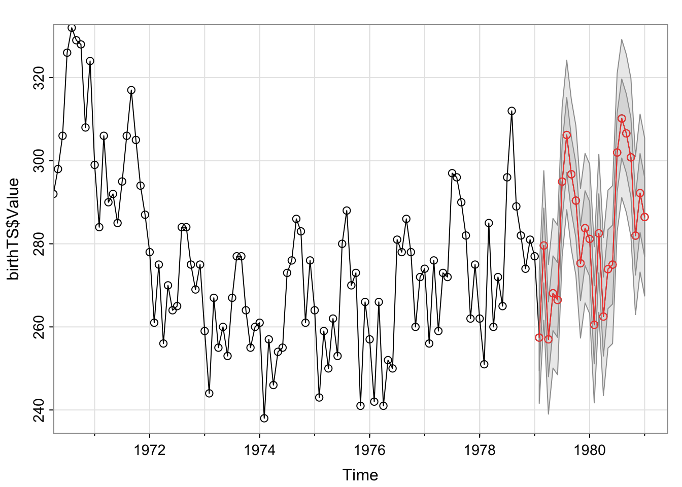
$pred
          Jan      Feb      Mar      Apr      May      Jun      Jul      Aug
1979          257.4217 279.5911 257.0032 268.0920 266.4857 294.9724 306.1982
1980 281.1732 260.4987 282.5277 262.4848 273.9019 274.9926 301.9751 310.1671
1981 286.4452
          Sep      Oct      Nov      Dec
1979 296.7487 290.3933 275.3080 283.7623
1980 306.5751 300.8098 281.9722 292.2112
1981

$se
          Jan      Feb      Mar      Apr      May      Jun      Jul      Aug
1979          7.923840 8.999167 8.999167 8.999167 8.999167 8.999167 8.999167
1980 8.999167 9.394536 9.506053 9.506053 9.506053 9.506053 9.506053 9.506053
1981 9.506053
          Sep      Oct      Nov      Dec
1979 8.999167 8.999167 8.999167 8.999167
1980 9.506053 9.506053 9.506053 9.506053
1981 The model is stated
\[Y_t = \delta + \phi_1Y_{t-1} + W_t\] where \(W_t \stackrel{iid}{\sim} N(0,\sigma^2_w)\) is independent Gaussian white noise with mean 0 and constant variance, \(\sigma^2_w\).
Expected Value
\[E(Y_t) = E(\delta + \phi_1 Y_{t-1} + W_t) = E(\delta) + E(\phi_1 Y_{t-1})+ E(W_t) \] \[= \delta + \phi_1 E( Y_{t-1}) + 0 \] \[= \delta + \phi_1 E( Y_{t})\]
if the process is stationary (constant expected value).
If we solve for \(E(Y_t)\), we get that \(E(Y_t) = \mu = \frac{\delta}{1-\phi_1}\).
Variance
By the independence of current error and \(Y_{t-1}\) (as \(Y_{t-1}\) is only a function of past errors),
\[Var(Y_t) = Var(\delta + \phi_1 Y_{t-1} + W_t) = Var(\phi_1 Y_{t-1} + W_t)\] \[= Var(\phi_1 Y_{t-1}) + Var(W_t)\] \[= \phi_1^2 Var( Y_{t-1}) + \sigma^2_w\]
\[= \phi_1^2 Var( Y_{t}) + \sigma^2_w\]
if the process is stationary.
If we solve for \(Var(Y_t)\), then we find that
\[Var(Y_t) = \frac{\sigma^2_w}{1-\phi_1^2}\]
Since \(Var(Y_t)>0\), then \(1-\phi_1^2 > 0\) and therefore \(|\phi_1| < 1\).
Covariance
Let’s assume that the data have a mean of 0 (we’ve removed the trend and seasonality) such that \(\delta = 0\) and \(Y_t = \phi_1Y_{t-1} + W_t\).
Then the \(Cov(Y_t,Y_{t-k}) = E(Y_tY_{t-k})\). For \(k=1\) (observations 1 time unit apart),
\[\Sigma_Y(1) = Cov(Y_t,Y_{t-1}) = E(Y_tY_{t-1}) = E((\phi_1Y_{t-1} + W_t)Y_{t-1}) \] \[= E(\phi_1Y_{t-1}^2 + W_tY_{t-1}) \] \[= \phi_1E(Y_{t-1}^2) + E(W_t)E(Y_{t-1}) \text{ since }Cov(W_t,Y_{t-1}) = 0\] \[= \phi_1Var(Y_{t-1}) + 0E(Y_{t-1})\] \[= \phi_1Var(Y_{t}) \]
Thus,
\[\rho_1 = Cor(Y_t,Y_{t-1}) = \frac{Cov(Y_t,Y_{t-1}) }{Var(Y_t)} = \frac{\phi_1Var(Y_t) }{Var(Y_t)} = \phi_1\]
For \(k>1\), multiple each side of the model by \(Y_{t-k}\) and take the expectation.
\[Y_t = \phi_1Y_{t-1} + W_t\]
\[Y_{t-k}Y_t = \phi_1Y_{t-k}Y_{t-1} + Y_{t-k}W_t\] \[E(Y_{t-k}Y_t) = E(\phi_1Y_{t-k}Y_{t-1}) + E(Y_{t-k}W_t)\]
\[Cov(Y_{t-k},Y_t) = \phi_1Cov(Y_{t-k},Y_{t-1}) \] \[\Sigma_Y(k) = \phi_1\Sigma_Y(k-1) \]
If we work recursively, starting with \(\Sigma_Y(1)\), we get
\[\Sigma_Y(1) = \phi_1\Sigma_Y(0) \] \[\Sigma_Y(2) = \phi_1\Sigma_Y(1) = \phi_1^2\Sigma_Y(0) \] \[\Sigma_Y(3) = \phi_1\Sigma_Y(2) = \phi_1^3\Sigma_Y(0) \]
\[\Sigma_Y(k) = \phi_1^k\Sigma_Y(0) \]
So the correlation for observations \(k\) lags apart is
\[\rho_k = \frac{\Sigma_Y(k) }{Var(Y_t)} = \frac{\phi_1^kVar(Y_t) }{Var(Y_t)} = \phi_1^k\]
\[Y_t = \delta + \phi_1Y_{t-1} + W_t\]
where \(t= ...,-3,-2,-1,0,1,2,3,...\)
By successive substitution, we can rewrite this model,
\[Y_t = \delta + \phi_1(\delta + \phi_1Y_{t-2} + W_{t-1}) + W_t =\delta(1 + \phi_1) + \phi_1^2Y_{t-2} + \phi_1W_{t-1} + W_t \] \[ =\delta(1 + \phi_1) + \phi_1^2(\delta + \phi_1Y_{t-3} + W_{t-2}) + \phi_1W_{t-1} + W_t \] \[=\delta(1 + \phi_1 + \phi_1^2) + \phi_1^3Y_{t-3} + \phi_1^2W_{t-2} + \phi_1W_{t-1} + W_t \] \[ =\delta(1 + \phi_1 + \phi_1^2 + \cdots) + W_t + \phi_1W_{t-1} +\phi_1^2W_{t-2} +\phi_1^3W_{t-3}+\cdots \]
Using infinite geometric series (\(\sum^\infty_{i=0}r^i = (1-r)^{-1}\) if \(|r|<1\)), the first part converges to \(\frac{\delta}{1-\phi_1}\) if \(|\phi_1|<1\). Similarly, the sum of random variables converges to a finite value when \(|\phi_1|<1\).
With this format, it is clear that for an AR(1) process,
\[E(Y_t) = E(\frac{\delta}{1-\phi_1} + W_t +\phi_1W_{t-1} + \phi_1^2 W_{t-2} + \cdots ) = \frac{\delta}{1-\phi_1}\]
\[Var(Y_t) = Var(\frac{\delta}{1-\phi_1} + W_t +\phi_1W_{t-1} + \phi_1^2 W_{t-2} + \cdots ) \] \[= \sigma^2_w(1+\phi_1^2 + \phi_1^4 + \cdots) \] \[ =\frac{\sigma^2_w}{1-\phi_1^2}\text{ if } |\phi_1|<1\]
Let \(h>0\), then
\[Cov(Y_t,Y_{t-h}) = Cov(\frac{\delta}{1-\phi_1} + W_t +\phi_1W_{t-1} + \phi_1^2 W_{t-2} + \cdots ,\frac{\delta}{1-\phi_1} + W_{t-h} +\phi_1W_{t-h-1} + \phi_1^2 W_{t-h-2} + \cdots ) \]
\[= Cov( W_t +\phi_1W_{t-1} + \phi_1^2 W_{t-2} + \cdots ,W_{t-h} +\phi_1W_{t-h-1} + \phi_1^2 W_{t-h-2} + \cdots ) \]
\[= \sum_{j = 0}^\infty Cov(\phi_1^{h+j}W_{t-h-j},\phi_1^{j} W_{t-h-j})\] \[= \sum_{j = 0}^\infty \phi_1^{h+2j}Var(W_{t-h-j}) \]
\[= \phi_1^h\sigma_w^2\sum_{j = 0}^\infty \phi_1^{2j} \] \[= \frac{\phi_1^h\sigma_w^2}{1-\phi_1^2}\text{ if } |\phi_1|<1\]
Thus,
\[Cor(Y_t,Y_{t-h}) = \frac{Cov(Y_t,Y_{t-h}) }{SD(Y_t)SD(Y_{t-h})} = \frac{\phi_1^h\sigma_w^2}{1-\phi_1^2}/\frac{\sigma^2_w}{1-\phi_1^2}\] \[= \phi_1^h\]
To supplement these notes, please check out the following time series textbooks for a more thorough introduction to the material.
“Time series: a data analysis approach using R” by Robert Shunway and David Stoffer (Shunway and Stoffer 2019)
“The Analysis of Time Series: An Introduction” by Christopher Chatfield (Chatfield and Xing 2019) is available at the Macalester Library.
“Time Series Analysis with Applications in R” by Jonathan Cryer and Kung-Sik Chan (Cryer and Chan 2008)