With correlated data, we often have repeated measures of some characteristic of a group of subjects or, more generally, of a set of units, collected with some random mechanism.
Before we collect data, we imagine those observations to be random variables.
Let’s make sure we are all on the same page with the probability concepts that are vital for us to understand the foundational models for correlated data.
2.1 Random Variable
A random variable is a variable whose value is subject to variation due to chance.
Note: Mathematically, a random variable\(X:\Omega\rightarrow E\)is a measurable function from the sample space set of possible random outcomes,\(\Omega\), to some set\(E\)where usually,\(E = \mathbb{R}\).
A discrete random variable is a random variable that can take only a countable number of distinct values (so the set \(E\) is countable).
Example: A Binomial random variable is a discrete random variable \(X\) where \(X\) can take values \(0,1,2,...,n\) and \(P(X = x) = {n \choose x} p^x(1-p)^{n-x}\)
Example: A Poisson random variable is a discrete random variable \(X\) where \(X\) can take values \(0,1,2,...\) and \(P(X = x) = \frac{\lambda^ke^{-\lambda}}{x!}\)
The distribution of a discrete random variable is described as a list of values and their associated probabilities, usually described with a probability mass function, \(p(x) = P(X = x)\).
A continuous random variable is a random variable that can take an uncountable (think infinite) number of distinct numerical values (the set \(E\) is a subset of \(\mathbb{R}\)).
The distribution of a continuous random variable is described with probabilities of intervals of values (rather than distinct values) through the cumulative distribution function (cdf), \(F(x) = P(X < x)\).
For most of the distributions we will talk about, the distribution can also be described with a probability density function (PDF) such that the cdf is defined as an integral over the pdf, \(F(x) = \int^x_{-\infty}f(y)dy\) where \(f(y) \geq 0\) is the pdf.
Example: Uniform distribution on \([a,b]\) where \(f(x) = \frac{1}{b-a} \text{ if } a\leq x \leq b; 0\text{ otherwise }\).
Example: Gaussian distribution on the real line, \(\mathbb{R}\), where \(f(x) = \frac{1}{\sigma\sqrt{2\pi}}e^{-\frac{1}{2}\left(\frac{x - \mu}{\sigma}\right)^2}\).
Example: Beta distribution on \([0,1]\) where \(f(x) = \frac{\Gamma(\alpha+\beta)}{\Gamma(\alpha)\Gamma(\beta)}x^{\alpha-1}(1-x)^{\beta-1}\).
2.2 Moments
2.2.1 Expectation
The expected value of a random variable is the long-run average and calculated as a weighted sum of possible values (weighted by the probability) \[\mu = E(X) = \sum_{\text{all }x}x\cdot P(X=x) \] for a discrete random variable and \[\mu = E(X) = \int_{-\infty}^{\infty}xf(x)dx \] for a continuous random variable where \(f(x)\) is the probability density function.
Properties
For random variables \(X\) and \(Y\) and constant \(a\), the following are true (you can show them using the definitions of expected value),
The covariance between two random variables is a measure of linear dependence (i.e., average product of how far you are from the mean or expected value in each variable). The theoretical covariance between two random variables, \(X\) and \(Y\), is
\[Cov(X,Y) = E((X - \mu_X)(Y-\mu_Y))\] where the means are defined as \(\mu_X = E(X)\) and \(\mu_Y = E(Y).\)
The variance is the covariance of a random variable with itself,
Covariance of a Sequence or Series of Random Variables
In this class, we will often work with a sequence or series of random variables that are indexed or ordered. Imagine we have a series of indexed random variables \(X_1,...,X_n\). The subscripts indicate the order. For any two of those random variables, \(X_l\) and \(X_k\), the covariances are defined as
\[Cov(X_l, X_k) = E((X_l - \mu_l)(X_k - \mu_k)) \] where \(\mu_l = E(X_l)\) and \(\mu_k = E(X_k).\)
Note: the order of the variables does not matter, \(Cov(X_l,X_k) = Cov(X_k,X_l)\), due to the commutative properties of multiplication.
Notation
We’ll use the Greek letter, sigma, \(\sigma\), to represent covariance. With a series of indexed random variables \(X_1,...,X_n\), we use the subscripts or indices on the \(\sigma\) as a short-hand for the covariance between those two random variables, \[\sigma_{lk} = Cov(X_l, X_k)\] where \(l,k \in \{1,2,...,n\}\).
If the index is the same, \(l = k\), then the covariance of the variable with itself is the variance, a measure of the spread of a random variable.
Let us denote the variance as \[\sigma_l^2 = Cov(X_l,X_l) = Var(X_l)\]
The standard deviation (SD) of \(X_l\) is the square root of the variance, \[\sigma_l = SD(X_l) = \sqrt{\sigma_l^2}\]We often interpret the standard deviation because the units of the SD are the units of the random variable and not in squared units.
Theorem: If \(X_l\) and \(X_k\) are independent, then \(Cov(X_l, X_k) = 0\). (See the technical note below to help you prove this.) The converse is not true.
Properties
For random variables \(X_l\), \(X_j\), \(X_k\) and constants \(a\), \(b\), and \(c\), the following are true (you can show them using the definitions),
\[Cov(aX_l, b X_k) = abCov(X_l,X_k)\]\[Cov(aX_l + c, b X_k) = abCov(X_l,X_k)\]
\[Cov(aX_l + b X_j, cX_k) = acCov(X_l,X_k) + bcCov(X_j,X_k)\]
Thus, we have the following properties of variance,
The standardized version of the covariance is the correlation. The theoretical correlation between two random variables is calculated by dividing the covariance by the standard deviations of each variable,
For a set of discrete random variables \((X_1,...,X_k)\), the joint probability mass function of \(X_1,...,X_k\) is defined as the function such that for every point \((x_1,...,x_k)\) in the \(k\)-dimensional space, \[p(x_1,...,x_k) = P(X_1 = x_1,...,X_k = x_k) \geq 0\]
If \((x_1,...,x_k)\) is not one of the possible values for the set of random variables, then \(p(x_1,...,x_k) = 0\). Since there can be at most countably many points with \(p(x_1,...,x_k)>0\) and since these points must account for all the probabilities, we know that \[\sum_{\text{all }(x_1,...,x_k)}p(x_1,...,x_k) = 1 \] and for a subset of points called \(A\), \[P((x_1,...,x_k)\in A ) = \sum_{(x_1,...,x_k)\in A}p(x_1,...,x_k) \]
The joint distribution function of a set of continuous random variables \((X_1,...,X_k)\) is defined in terms of the cumulative joint distribution function, \[F(x_1,...,x_k) = P(X_1 < x_1,...,X_k < x_k)\]
For a set of continuous random variables \((X_1,...,X_k)\), the joint density function of \(X_1,...,X_k\) is defined as the non-negative function defined for every point \((x_1,...,x_k)\) in the \(k\)-dimensional space such that for every subset \(A\) of the space, \[P((x_1,...,x_k)\in A ) = \int\dots\int_A f(x_1,...,x_k) dx_1...dx_k\]
In order to be a joint probability density function, \(f\) must be a non-negative function and \[\int_{-\infty}^{\infty}\cdots\int_{-\infty}^{\infty}f(x_1,...,x_k) dx_1...dx_k= 1 \]
2.3.0.1 Technical Note
For two discrete random variables, the covariance can be written as \[Cov(X_l,X_k) = \sum_{\text{all }x_l}\sum_{\text{all }x_k} (x_l -\mu_l)(x_k -\mu_k)p_{lk}(x_l,x_k) \] where \(p_{lk}(x_l,x_k)\) is the joint probability distribution such that \(p_{lk}(x_l,x_k) = P(X_l = x_l \text{ and }X_k = x_k)\) and \(\sum_{\text{all }x_l}\sum_{\text{all }x_k}p_{lk}(x_l,x_k)=1\).
For two continuous random variables, the covariance can be written as \[Cov(X_l,X_k) = \int^\infty_{-\infty}\int^\infty_{-\infty} (x_l -\mu_l)(x_k -\mu_k)f(x_l,x_k)dx_ldx_k \] where \(f(x_l,x_k)\) is the joint density function such that \(\int^\infty_{-\infty}\int^\infty_{-\infty}(x_l,x_k)dx_ldx_k=1\). We’ll see some examples of joint densities soon.
Two random variables are said to be statistically independent if and only if \[f(x_l,x_k) = f_{l}(x_l)f_k(x_k) \] for all possible values of \(x_l\) and \(x_k\) for continuous random variables and \[P(X_l = x_l, X_k = x_k)=P(X_l=x_l)P(X_k=x_k) \] for discrete random variables.
A finite set of random variables is said to be mutually statistically independent if and only if \[f(x_1,x_2,...x_k) = f_{1}(x_1)\cdots f_k(x_k) \] for all possible values for continuous random variables and \[P(X_1 = x_1,X_2 = x_2,..., X_k = x_k)=P(X_1=x_1)P(X_2=x_2)\cdots P(X_k=x_k)\] for discrete random variables.
Matrix notation can help us organize distributional information about the set of random variables.
2.4.1 Random Vectors
A random vector is a vector (a collection) of \(m\) indexed random variables such that \[\mathbf{X} = \left(\begin{array}{c} X_{1}\\ X_{2}\\ \vdots\\\\ X_{m}\\
\end{array}\right)\]
The expected value of a random vector \(\mathbf{X}\), written as \(E(\mathbf{X})\), is a vector of expected values, \[\boldsymbol{\mu} = E(\mathbf{X}) = \left(\begin{array}{c} E(X_1)\\ E(X_2)\\ \vdots\\ E(X_m) \end{array} \right)= \left(\begin{array}{c} \mu_1\\ \mu_2\\ \vdots\\ \mu_m \end{array} \right) \] where \(E(X_1) = \mu_1\),…,\(E(X_m) = \mu_m\)
The covariances of all pairs of values in a random vector \(\mathbf{X}\) can be organized in a covariance matrix,
using the notation introduced above that \(\sigma^2_l = Var(X_l)\) and \(\sigma_{lk} = Cov(X_l,X_k)\). We’ll talk much more about the covariance matrix.
2.4.2 Random Matrices
Let \(X_{ij}\) be an indexed random variable where index \(i=1,...,n\) refers to different subjects (different units) and the index \(j = 1,...,m\) refers to different observations over time or space. We can organize these variables in random vectors and then into a matrix for convenience.
The random matrix\(\mathbf{X}\) is written as \[\mathbf{X} = \left(\begin{array}{cccc} X_{11}&X_{12}&\cdots&X_{1m}\\ X_{21}&X_{22}&\cdots&X_{2m}\\ \vdots&\vdots&\ddots&\vdots\\ X_{n1}&X_{n2}&\cdots&X_{nm}\\
\end{array}\right) \] in which each column represents one observation time and the rows represent the \(n\) subjects or individual units.
The expected value of a random matrix \(\mathbf{X}\), written as \(E(\mathbf{X})\), is a matrix of expected values, \[E(\mathbf{X}) = \left(\begin{array}{cccc} E(X_{11})&E(X_{12})&\cdots&E(X_{1m})\\ E(X_{21})&E(X_{22})&\cdots&E(X_{2m})\\ \vdots&\vdots&\ddots&\vdots\\ E(X_{n1})&E(X_{n2})&\cdots&E(X_{nm}) \end{array} \right)\]
2.4.2.1 Properties
For random matrices or vectors of the same size \(\mathbf{X}\) and \(\mathbf{Y}\) and constant (not random) compatible matrices or vectors \(\mathbf{A}\) and \(\mathbf{B}\), the following are true,
Note: We will use bold typeface for random vectors and matrices and normal typeface for random variables.
2.5 Multivariate Normal Distribution
The normal probability density function for random variable \(X\) with mean \(\mu\) and standard deviation \(\sigma\) is \[ f(x) = \frac{1}{\sqrt{2\pi\sigma^2}}\exp\left(-\frac{1}{2}\left(\frac{x - \mu}{\sigma}\right)^2\right)\] Note: \[\left(\frac{x - \mu}{\sigma}\right)^2 = (x-\mu)(\sigma^2)^{-1}(x-\mu) \]
The multivariate normal probability density function for a k-dimensional random vector \(\mathbf{X} = (X_1,...,X_k)\) with mean vector \(\boldsymbol\mu\) and covariance matrix \(\boldsymbol\Sigma\) is \[ f(\mathbf{x}) = \frac{1}{(2\pi)^{k/2}|\boldsymbol\Sigma|^{1/2}}\exp\left(-\frac{1}{2}(\mathbf{x} - \boldsymbol\mu)^T\boldsymbol\Sigma^{-1}(\mathbf{x} - \boldsymbol\mu)\right)\]
Example - Bivariate Normal
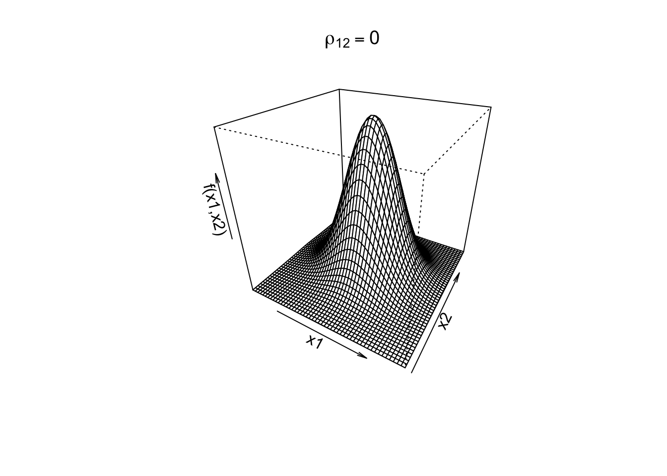
When \(k=2\), our random vector includes \(X_1\) and \(X_2\). Let \(\rho_{12}\) be the correlation between the two variables \(X_1\) and \(X_2\).
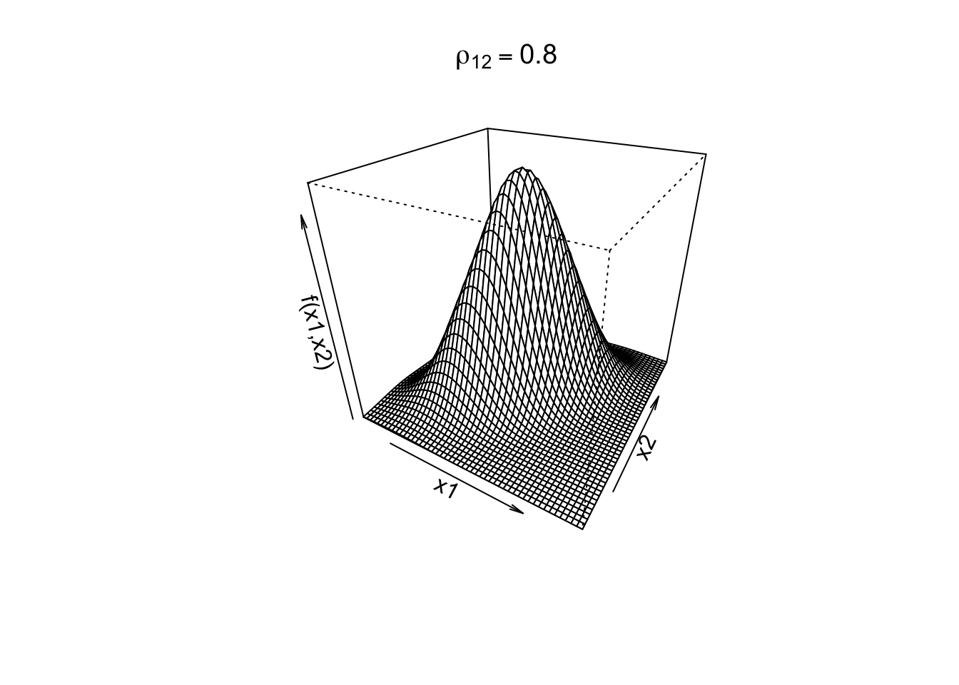
See below for 3D plots of the bivariate density function under two correlation values (\(\rho_{12}=0\) indicating no correlation and \(\rho_{12} = 0.8\) indicating a strong positive correlation) with standardized assumptions for the variance and mean, \(\sigma_1^2=\sigma^2_2 = 1\) and \(\mu_1=\mu_2=0\).
rho <-0bivn <- MASS::mvrnorm(5000, mu =c(0, 0), Sigma =matrix(c(1, rho, rho, 1), nrow =2))bivn.kde <- MASS::kde2d(bivn[,1], bivn[,2], h =2, n =50) #density function values (we'll discuss this function later)persp(bivn.kde, phi =30, theta =30,xlab='x1',ylab='x2',zlab='f(x1,x2)',main =expression(rho[12] ==0))
rho <-0.8bivn <- MASS::mvrnorm(5000, mu =c(0, 0), Sigma =matrix(c(1, rho, rho, 1), nrow =2))bivn.kde <- MASS::kde2d(bivn[,1], bivn[,2], h =2, n =50)persp(bivn.kde, phi =30, theta =30,xlab='x1',ylab='x2',zlab='f(x1,x2)',main =expression(rho[12] ==0.8))
2.5.1 Contours of Density
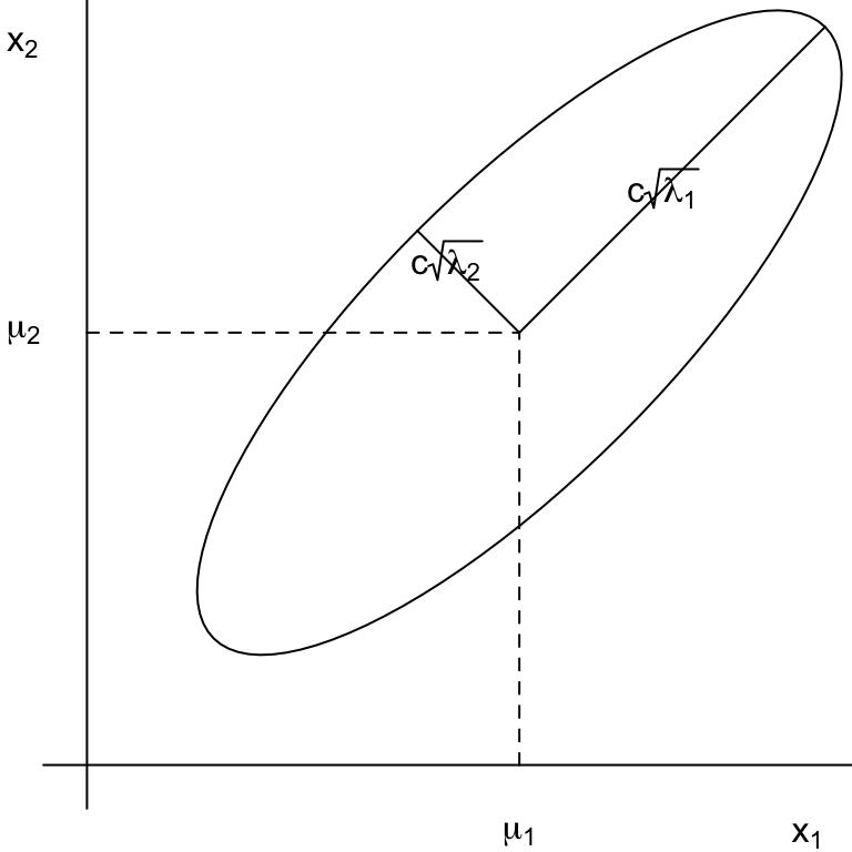
The multivariate normal density function is constant on surfaces where the square of the Mahalanobis-type distance \((\mathbf{x} - \boldsymbol\mu)^T\boldsymbol\Sigma^{-1}(\mathbf{x} - \boldsymbol\mu)\) is constant and these are called contours.
The contours are ellipsoids defined by \[(\mathbf{x} - \boldsymbol\mu)^T\boldsymbol\Sigma^{-1}(\mathbf{x} - \boldsymbol\mu) = c^2\] such that the ellipsoids are centered at \(\boldsymbol\mu\) and have axes \(\pm c\sqrt{\lambda_{i}}\mathbf{e}_i\) where \(\boldsymbol\Sigma \mathbf{e}_i = \lambda_i\mathbf{e}_i\) for \(i=1,...,k\). Thus, \(c\sqrt{\lambda_{i}}\) are the radii of the axes (\(\lambda_i\) are eigenvalues of \(\boldsymbol\Sigma\)) and the eigenvectors \(\mathbf{e}_i\) are the directions of the axes.
Also, in this context, \(c\) is the Mahalanobis distance between points in this distribution. We may refer to \(c\) as the radius, but note that this is the radius of the ellipse only when it is a circle and \(\lambda_{i}=1\).
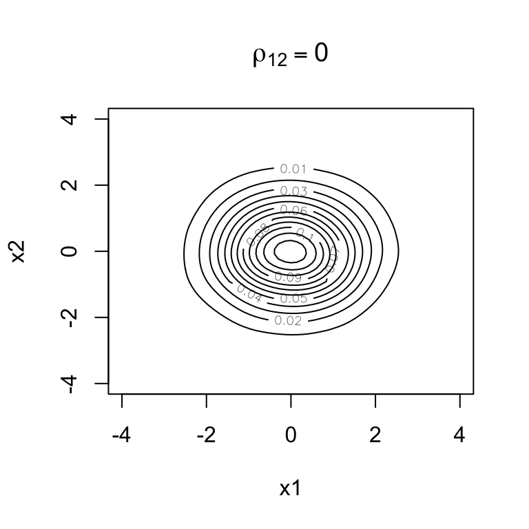
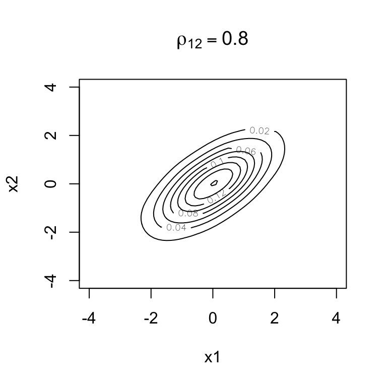
Below are contours of bivariate normal density functions with the values representing the density function (height).
rho =0bivn <- MASS::mvrnorm(5000, mu =c(0, 0), Sigma =matrix(c(1, rho, rho, 1), 2))bivn.kde <- MASS::kde2d(bivn[,1], bivn[,2], h =2, n =50)contour(bivn.kde,xlab='x1',ylab='x2',main =expression(rho[12] ==0),xlim=c(-4,4),ylim=c(-4,4))
rho =0.8bivn <- MASS::mvrnorm(5000, mu =c(0, 0), Sigma =matrix(c(1, rho, rho, 1), 2))bivn.kde <- MASS::kde2d(bivn[,1], bivn[,2], h =2, n =50)contour(bivn.kde,xlab='x1',ylab='x2',main =expression(rho[12] ==0.8),xlim=c(-4,4),ylim=c(-4,4))
These should look familiar if you looked at a topographic map for hiking in mountainous areas.
2.5.2 Properties of Multivariate Normal
Linear Combinations
If \(\mathbf{X}\) is distributed as a k-dimensional normal distribution with mean \(\boldsymbol\mu\) and covariance \(\boldsymbol\Sigma\), then any linear combination of variables (where \(\mathbf{a}\) is a vector of constants), \(\mathbf{a}^T\mathbf{X} = a_1X_1+a_2X_2+\cdots+a_kX_k\) is distributed as normal with mean \(\mathbf{a}^T\boldsymbol\mu\) and covariance \(\mathbf{a}^T\boldsymbol\Sigma\mathbf{a}\)
Chi-Squared Distribution The chi-squared distribution with \(k\) degrees of freedom is the distribution of the sum of the squares of \(k\) independent standard normal random variables. You typically prove this is true in Probability.
Theorem: If a random vector \(\mathbf{X}\in\mathbb{R}^k\) follows a multivariate normal distribution with mean \(\boldsymbol\mu\) and covariance \(\boldsymbol\Sigma\), then \((\mathbf{X} - \boldsymbol\mu)^T\boldsymbol\Sigma^{-1}(\mathbf{X} - \boldsymbol\mu)\) follows a Chi-squared distribution with \(k\) degrees of freedom.
Sketch of proof: Using the Cholesky decomposition, we get \(\boldsymbol\Sigma = \mathbf{L}\mathbf{L}^T\). Then define a random vector \(\mathbf{Y}\) such that \[\mathbf{Y} = \mathbf{L}^{-1}(\mathbf{X} - \boldsymbol{\mu})\] Show that \(\mathbf{Y}\) is a vector of independent standard normal random variables. You can use the properties of linear combinations above.
Then show that we have a sum of independent standard normals, \[(\mathbf{X} - \boldsymbol\mu)^T\boldsymbol\Sigma^{-1}(\mathbf{X} - \boldsymbol\mu) = \mathbf{Y}^T\mathbf{Y} = \sum Y_i^2\]
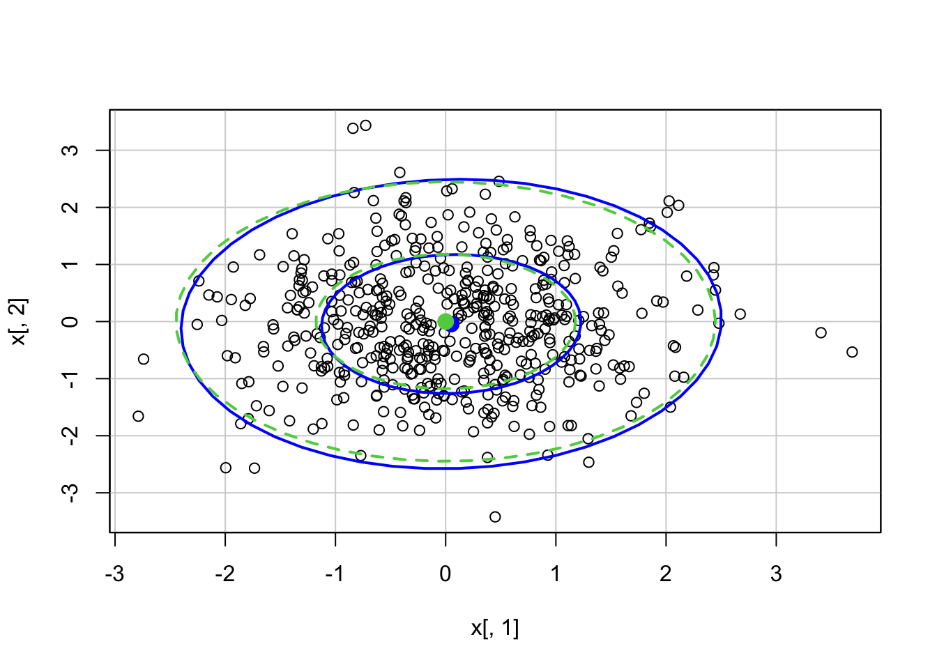
Extensions of Intervals to Multiple Dimensions - Ellipse Percentiles Now that we know about the contours of a multivariate normal distribution and we know the probability distribution for the contours, we can extend the ideas of intervals (such as confidence intervals or intervals of uncertainty) to a multivariate situation.
The contours containing \(\alpha\) of the probabilities under the multivariate normal distribution are the values of \(\mathbf{x}\) that satisfy \[(\mathbf{x} - \boldsymbol\mu)^T\boldsymbol\Sigma^{-1}(\mathbf{x} - \boldsymbol\mu) = \chi^2_k(\alpha)\] where \(\chi^2_k(\alpha)\) is the \(\alpha \cdot 100\) percentile of a chi-squared distribution with \(k\) degrees of freedom. Therefore, \[P((\mathbf{x} - \boldsymbol\mu)^T\boldsymbol\Sigma^{-1}(\mathbf{x} - \boldsymbol\mu) \leq \chi^2_k(\alpha)) = \alpha\]
That means that we can calculate ellipses that correspond to a probability of say \(\alpha = 0.95\), for example (probability = volume under the surface). In a univariate situation, these ellipses correspond to intervals such that the area under the curve equals the probability of 0.95.
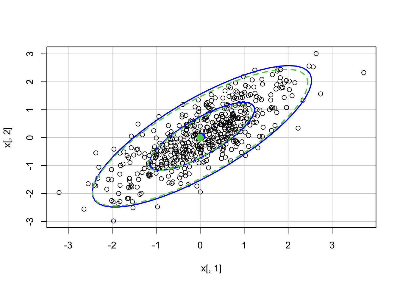
For a bivariate normal with mean vector (0,0), variances equal to 1, and correlation equal to 0 (and then 0.8), there is R code below to calculate the 0.5 and 0.95 ellipses based on the theoretical mean and covariance (green lines) or estimated based on sample data (red lines).
x <- MASS::mvrnorm(500, mu =c(0,0), Sigma =matrix(c(1,0,0,1),2))tmp <- car::dataEllipse(x[,1],x[,2]) #based on datac2 <-qchisq(.5,df =2)car::ellipse(c(0,0), matrix(c(1,0,0,1),2),sqrt(c2), col=3, lty=2) #theoreticalc2 <-qchisq(.95,df =2)car::ellipse(c(0,0), matrix(c(1,0,0,1),2),sqrt(c2), col=3, lty=2)
x <- MASS::mvrnorm(500, mu =c(0,0), Sigma =matrix(c(1,.8,.8,1),2))tmp <- car::dataEllipse(x[,1],x[,2]) #based on datac2 <-qchisq(.5,df =2)car::ellipse(c(0,0), matrix(c(1,.8,.8,1),2),sqrt(c2), col=3, lty=2) #how we generated datac2 <-qchisq(.95,df =2)car::ellipse(c(0,0), matrix(c(1,.8,.8,1),2),sqrt(c2), col=3, lty=2)