For this course, all of the methods we discuss have a way to model the inherent dependence in the data, directly or indirectly. Ultimately, they are modeling the covariance of pairs of random variables. Before we discuss models for a specific data type, let’s think about modeling covariance more generally.
In previous sections, we discussed a random vector, a set of random variables. These random variables could represent different quantities or characteristics. We hinted that these variables could be ordered or indexed in some way.
We will formalize that here. We focus now on a random process, a series of random variables representing the same characteristic ordered or indexed by time or space.
3.1 Random Process
A random process is a series of random variables indexed by time or space, \(\{Y_t\}_{t\in T}\), defined over a common probability space. We can organize a finite set of these variables in a random vector,
For time series data, the set of indices \(T=\{0,1,2,...,n\}\) indicates the time ordering of the random variables.
For longitudinal data, we index our data for one unit/subject with a random process where \(T = \{1,2,...,m\}\) indicates the ordering of the repeated random variables over time.
For spatial data, \(T\) refers to a set of points in space measured by (longitude, latitude).
Key Point: A random process can capture how a characteristic evolves over time (or space or both), and \(Y\) represents the random value of that characteristic.
3.2 Autocovariance
Remember that the covariance between two random variables, \(X\) and \(Y\), is defined as
The covariance values range over the entire real line \((-\infty,\infty)\).
3.2.1 Autocovariance Function
For a random process \(\{Y_t\}_{t\in T}\), we can summarize the covariance between two random variables in the process with different indices, \(Y_t\) and \(Y_s\), as a function of the times/spaces, \(t\) and \(s\). The autocovariance function of \(s\) and \(t\) is the covariance of the random variables at those times/spaces,
For times series, \(t\) and \(s\) will be integer indices of time.
For longitudinal data, \(t\) and \(s\) will refer to observations times.
For spatial data, \(t\) and \(s\) will be points in space, (longitude, latitude).
Throughout this course, we’ll use the capital Greek letter Sigma, \(\Sigma\), to denote covariance. We’ll use it in a few different ways, but it will always refer to covariance.
For example, we can refer to the covariance between the first and second random variable with \(\Sigma_Y(1,2)\) and the covariance between the second and fourth with \(\Sigma_Y(1, 4)\). We’ll come back to thinking about simplifying this autocovariance function.
3.2.2 Autocorrelation Function
In general, correlation is easier to interpret than covariance since correlation values are restricted to be between -1 and 1 (inclusive).
Remember that the correlation of two random variables \(X\) and \(Y\) is defined as
We use \(\rho\) to notate theoretical correlation (in contrast to \(r\), which refers to the sample correlation coefficient).
For example, we can refer to the correlation between the first and second random variable with \(\rho_Y(1,2)\) and the correlation between the second and fourth with \(\rho_Y(1, 4)\). Again, we’ll come back to thinking about simplifying this autocorrelation function.
3.2.3 Covariance Matrix
If we have \(m\) random variables \(\mathbf{Y} = (Y_1,...,Y_m)\) of a random process, we might be interested in knowing the covariance between every pair of indexed variables. We could plug the indices into the autocovariance function. The covariance between the \(i\)th observation and the \(j\)th observation in the process would be
\[\sigma_{ij} = \Sigma_Y(i, j)\]
Among the \(m\) variables, there are \(m(m-1)/2\) unique pair-wise covariances and \(m\) variances and they could be organized into a \(m\times m\) symmetric covariance matrix,
\[\boldsymbol{\Sigma}_Y = Cov(\mathbf{Y}) = \left(\begin{array}{cccc}\sigma^2_1&\sigma_{12}&\cdots&\sigma_{1m}\\\sigma_{21}&\sigma^2_2&\cdots&\sigma_{2m}\\\vdots&\vdots&\ddots&\vdots\\\sigma_{m1}&\sigma_{m2}&\cdots&\sigma^2_m\\ \end{array} \right) \] where \(\sigma^2_i = \sigma_{ii}\). Note that \(\sigma_{ij} = \sigma_{ji}\).
The covariance matrix can also be written using the definitions of covariance and the properties of matrix algebra as
This is an important property because it gives us the covariance of a linear combination of our random process values: \(\mathbf{A}\mathbf{Y}\). This is also very useful when working with regression estimates (we’ll come back to this).
3.2.3.2 Positive Semidefiniteness
For the autocovariance function to be valid, it must be positive semidefinite. We can check this by evaluating it at any set of \(m\) indices and checking to see if the resulting covariance matrix is positive semidefinite. A symmetric matrix, \(\boldsymbol{\Sigma}\), is positive semidefinite if and only if
\[\mathbf{x}^T\boldsymbol{\Sigma}\mathbf{x} \geq 0\text{ for all }\mathbf{x}\in \mathbb{R}^m\] or equivalently,
\[\text{The eigenvalues of }\boldsymbol{\Sigma}\text{ are all }\geq 0\]
In practice, this is important to be aware of when modeling covariance, as the covariance matrix must be positive semidefinite.
To ensure this matrix is positive semidefinite, we could use the Cholesky Decomposition in the modeling process because the decomposition is only valid for positive definite (\(>\) instead of \(\geq\) in the definitions above) matrices,
\[ \boldsymbol{\Sigma} = \mathbf{LL}^T\]
where \(\mathbf{L}\) is a lower triangular matrix (upper diagonal is all 0), we’ll return to this.
3.2.4 Correlation Matrix
If we have \(m\) random variables \(Y = (Y_1,...,Y_m)\), we might be interested in knowing the autocorrelation between every pair of observations. The correlation between the \(i\)th observation and the \(j\)th observation would be
\[\rho_{ij} = \rho_Y(i, j)\]
These \(m(m-1)/2\) correlations could be organized into a \(m\times m\) symmetric correlation matrix,
If you have the covariance matrix \(\boldsymbol{\Sigma}\), you can extract the correlation matrix,
\[\mathbf{R}_Y = \mathbf{D}^{-1}\boldsymbol{\Sigma}_Y\mathbf{D}^{-1}\] where \(\mathbf{D} = \sqrt{diag(\boldsymbol{\Sigma}_Y)}\), a diagonal matrix with standard deviations along the diagonal because
We’ve been discussing covariance and correlation in terms of probability theory so far. What about if we have data?!
We need replicates to estimate any parameter (mean, covariance, correlation, etc.). For the covariance of pairs of variables, that means we need either:
multiple realizations of a random process (which could be multiple subjects), OR
simplifying assumptions about the structure of the autocovariance function.
3.3.1 Common Constraints
When we model covariance, we often make simplifying assumptions and use model constraints to estimate the covariance from the data. Below are some of the common constraints or assumptions we use. Like any assumption, we should check that it is a valid assumption to make with a dataset before reporting on the conclusions of the model.
3.3.1.1 Weak Stationarity
If the autocovariance function of a random process only depends on the difference in time/space, \(s-t\) (e.g., covariance depends only on the difference in observation times and not time itself), then we say that the autocovariance is weakly stationary, such that
\[\Sigma_Y(t, s) = \Sigma_Y(s-t)\] For example, this means that the covariance between the 1st and 4th observation is the same as the 2nd and 5th, 3rd and 6th, etc. This simplifies our function as we only need to know the difference in time/space rather than the exact time/space.
Additionally, a random process that is weakly stationary has a constant mean, \(\mu = E(Y_t) = E(Y_s)\), and constant variance, \(\sigma^2=Var(Y_t) = Var(Y_s)\). When we use the term “stationary” from now on, we refer to a “weak stationary” process.
Autocovariance (and autocorrelation) Function is only a function of the vector difference in time/space
In a covariance matrix, the constant variance of stationarity, \(\sigma_{i}^2 = \sigma^2\), means that we can write the covariance matrix as the variance times correlation matrix,
\[\boldsymbol{\Sigma}_Y = \sigma^2\mathbf{R}_Y\] where \(\mathbf{R}_Y\) is the correlation matrix.
Additionally, with the stationary assumption, the correlation matrix can be written in terms of the vector difference in time/space, similar to the covariance matrix.
If we are considering spatial data where space is defined by longitude and latitude, a weakly stationary process means that the covariance depends on the difference between two points in space, which is defined by both the distance (as the crow flies Euclidean distance) and the direction (e.g., a point on a compass such as NE or West or defined as the angle degrees from North). In linear algebra terminology, the difference is the vector difference.
3.3.1.2 Isotropy
A stronger assumption than weak stationarity is that the autocovariance function depends only on the distance in time/space, \(||s-t||\).
If this is true, then we typically say that the autocovariance function and random process are isotropic, such that the dependence doesn’t change as a function of the angle of the difference in space (NE v. West) but just the vector distance or vector norm. That is, \[\Sigma_Y(t, s) = \Sigma_Y(||s-t||)\]
Notes:
This distinction only applies to spatial data in which our index is a vector of length two or more.
Many spatial models we will use assume an isotropic covariance function.
3.3.1.3 Intrinsic Stationarity
If assuming a process is weak stationary is too strong a constraint, a slightly weaker constraint is that a random process is intrinsic stationary if
\[Var(Y_{s+h} - Y_s)\text{ depends only on h}\] meaning that the variance of the difference of random variables only depends on the vector difference, \(h\), in time or space.
This is similar to the concept of weak stationarity, but weak stationarity implies intrinsic stationarity, but not vice versa.
3.3.2 Common Model Structures
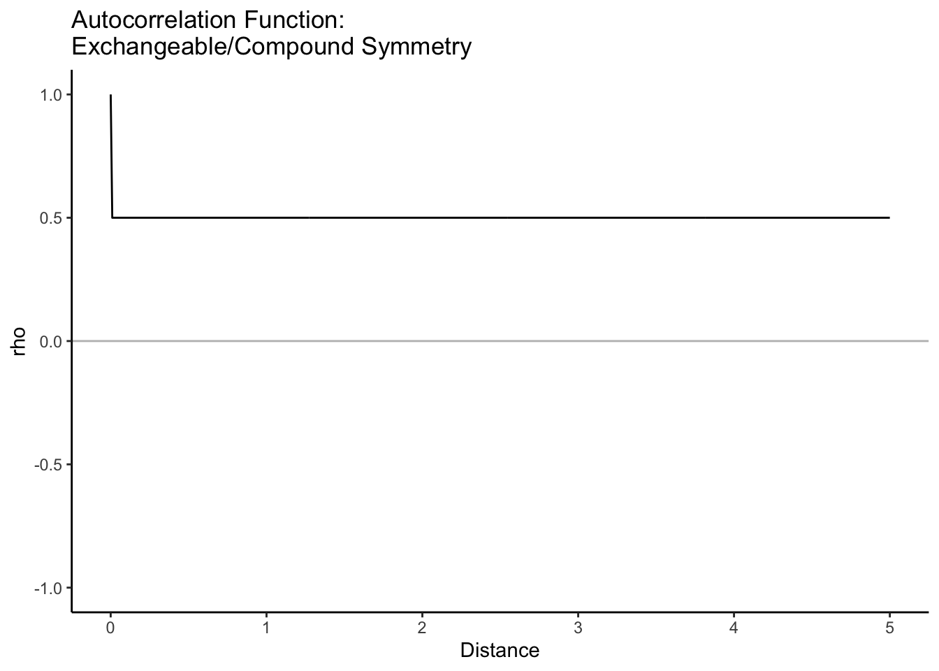
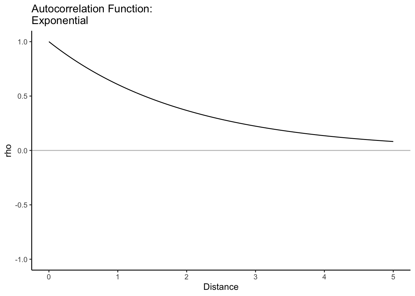
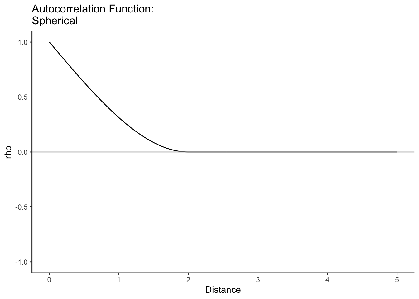
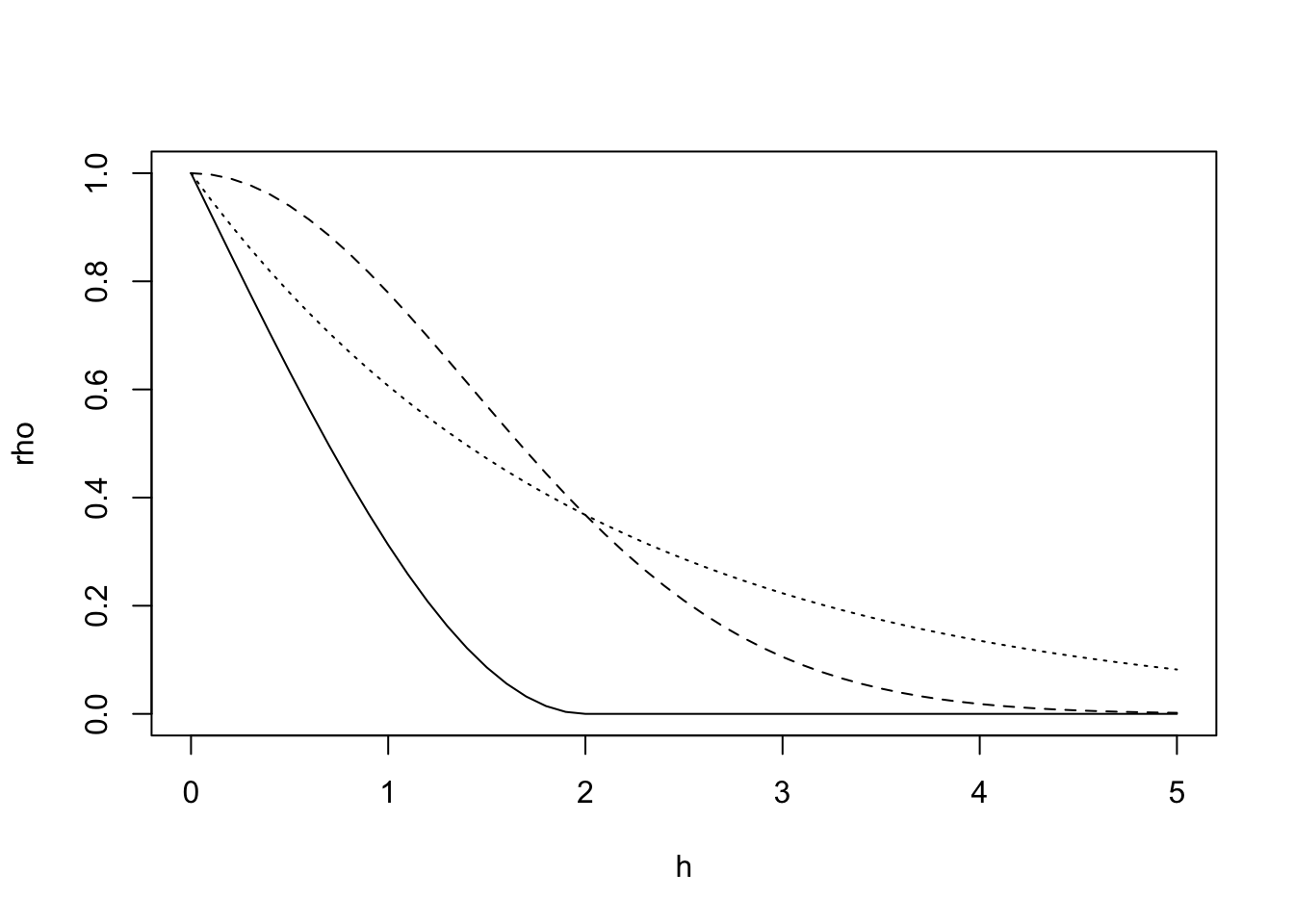
Here are some common correlation functions that are all weakly stationary and isotropic:
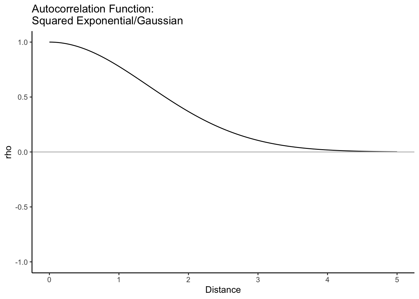
The correlation between two random variables decays (slightly different decay exponentially) to 0 as the difference in time/space increases. It decays more slowly than exponentially for differences < \(\phi\), but for differences > \(\phi\), it decays faster.
\[\rho_Y(s-t) = e^{-(||s-t||/\phi)^2}\] where \(\phi > 0\)
Let’s look at the last three on the same graph. With the same value of \(\phi\), the correlation function can look quite different.
h =seq(0,5,by=.1) #distancephi =2rho =rep(0, length(h))rho[h<phi] =1-1.5*(h[h<phi]/phi) +0.5*(h[h<phi]/phi)^3rho2 =exp(-(h/phi)^2)rho3 =exp(-h/phi)plot(h, rho, type ='l', ylim=c(0,1))lines(h, rho2, lty=2)lines(h, rho3, lty=3)
3.4 Estimating with Data
In this chapter, we have discussed the theory around autocovariance in function and matrix format and models, simplifications, and constraints that can be imposed and assumed.
In this last section, we’ll introduce the idea of estimating the numerical values of covariance and correlation based on data after assuming models, simplifications, and constraints.
The three estimators mentioned below can be used outside a larger statistical model, so we’ll start here.
3.4.1 Sample Covariance Matrix
To estimate the covariance matrix, \(\boldsymbol\Sigma\), with observed data sampled from the larger population as \(n\) realizations of these \(m\) random variables (imagine \(n\) individual people with \(m\) observations over time), we can calculate the sample covariance matrix,
\[\mathbf{S}_Y = \frac{1}{n-1}\sum^n_{i=1} (\mathbf{y}_i - \bar{\mathbf{y}})(\mathbf{y}_i - \bar{\mathbf{y}})^T \] where \(\mathbf{y}_i = (y_{i1},y_{i2},...,y_{im})\) and \(\bar{\mathbf{y}} = n^{-1} \sum^n_{i=1} \mathbf{y}_i\).
Therefore, the sample variances (on the diagonal of \(\mathbf{S}_Y\)) are the familiar estimates we saw in our introductory course,
Note: This estimation is only possible for longitudinal data if we observed \(m\) repeated measurements for each case at the same time. We typically don’t have more than one realization of the process for time series and spatial data. For longitudinal data, if we have unbalanced data collected at irregular times, we’ll need to use one of the common model structures to estimate the covariance. In the Longitudinal Data chapter, we’ll return to this.
3.4.2 Sample Autocovariance Function
If we assume that observed data come from a stationary process, we can estimate the autocovariance function with the sample autocovariance function (ACVF),
\[c_k = \frac{1}{n}\sum^{n-|k|}_{t=1}(y_t - \bar{y})(y_{t+|k|} - \bar{y})\] where \(\bar{y}\) is the sample mean, averaged across time/space, because we are assuming it is constant.
For any sequence of observations of the random process, \(y_1,...,y_n\), the estimated ACVF has the following properties:
If we assume that observed data come from a stationary process (or at least an intrinsic stationary process), we can estimate the semivariogram,
\[\gamma(h) = \frac{1}{2}Var(Y_{s+h} - Y_s)\]
To estimate the semivariogram, let \(H_1,...,H_k\) be a partition of the space of possible distances or lags \(h\), with \(h_u\) being a representative spatial lag/distance in \(H_u\). Then use your stationary process \(y_t\) to estimate the sample/empirical semivariogram.