library(tidyverse)

hikes <- read.csv("https://mac-stat.github.io/data/high_peaks.csv")14 Mid-semester review
Help each other with the following:
- Prepare to take notes. Open the activity qmd file.
TODAY’S GOALS
- Review the basics of wrangling and visualization
14.1 Warm-up
Thus far, we’ve learned how to:
- use
ggplot()to construct data visualizations - do some wrangling:
arrange()our data in a meaningful order- subset the data to only
filter()the rows andselect()the columns of interest mutate()existing variables and define new variablessummarize()various aspects of a variable, both overall and by group (group_by())
- reshape our data to fit the task at hand (
pivot_longer(),pivot_wider()) join()different datasets into one
Let’s review some basics, emphasizing some themes in Homework 3 feedback!
Along the way, pay special attention to formatting your code: code is communication.
EXAMPLE 1: Make a plot
Recall our data on hiking the “high peaks” in the Adirondack Mountains of northern New York state. This includes data on the hike’s highest elevation (feet), vertical ascent (feet), length (miles), time in hours that it takes to complete, and difficulty rating.
Construct a plot that allows us to examine how vertical ascent varies from hike to hike.
EXAMPLE 2: What’s wrong?
Critique the following interpretation of the above plot:
“The typical ascent is around 3000 feet.”
EXAMPLE 3: Captions, axis labels, and titles
Critique the use of the axis labels, caption, and title here. Then make a better version.
ggplot(hikes, aes(x = ascent)) +
  geom_density() +
  labs(x = "the vertical ascent of a hike in feet",
       title = "Density plot of hike vertical ascent")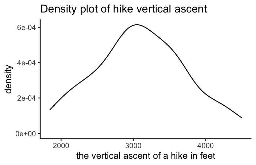
EXAMPLE 4: Wrangling practice – one verb
# How many hikes are in the dataset?


# What's the maximum elevation among the hikes?


# How many hikes are there of each rating?


# What hikes have elevations above 5000 ft?
EXAMPLE 5: Wrangling practice – multiple verbs
# What's the average hike length for each rating category?


# What's the average length of *only* the easy hikes


# What 6 hikes take the longest time to complete?


# What 6 hikes take the longest time per mile?
14.2 Midterm assessment
We will have a quiz next Tuesday, one week from today. Unlike the course project which will assess your deeper conceptual understanding of the course material, and your ability to build upon this in new settings, the quiz will assess your grasp on the foundations (eg: wrangling and visualization code and output).
Preparing for and completing this assessment is important to solidifying your understanding of these foundations before moving on to our final unit and course project.
Content
The quiz will cover activities 1-11, as labeled on the online course manual.
In general, the exercises will cover a variety of angles. For example…
What does this result mean in context?
You’ll be given some visualization / wrangling results and asked to interpret them.What code is necessary to completing the task at hand?
You’ll be given a task and asked for the necessary code.What does this code do?
You’ll be given some code without output and asked to anticipate the result.
Structure
Review the quiz practice for details.
14.3 Solutions
Click for Solutions
EXAMPLE 1: Make a plot
# A boxplot or histogram could also work!
ggplot(hikes, aes(x = ascent)) +
  geom_density()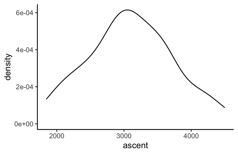
EXAMPLE 2: What’s wrong?
That interpretation doesn’t say anything about the variability in ascent or other important features.
EXAMPLE 3: Captions, axis labels, and titles
The axis label is too long, and the caption and title are redundant.
# Better
ggplot(hikes, aes(x = ascent)) +
  geom_density() +
  labs(x = "vertical ascent (feet)")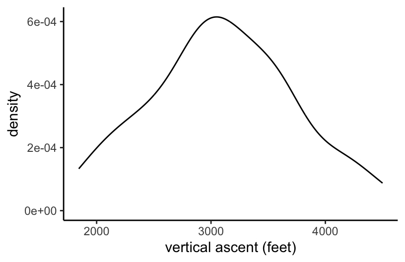
EXAMPLE 4: Wrangling practice – one verb
# How many hikes are in the dataset?
hikes %>%
  nrow()
## [1] 46

# What's the maximum elevation among the hikes?
hikes %>%
  summarize(max(elevation))
##   max(elevation)
## 1           5344

# How many hikes are there of each rating?
hikes %>%
  count(rating)
##      rating  n
## 1 difficult  8
## 2      easy 11
## 3  moderate 27

# What hikes have elevations above 5000 ft?
hikes %>%
  filter(elevation > 5000)
##              peak elevation difficulty ascent length time   rating
## 1     Mt. Marcy        5344          5   3166   14.8   10 moderate
## 2 Algonquin Peak       5114          5   2936    9.6    9 moderate
EXAMPLE 5: Wrangling practice – multiple verbs
# What's the average hike length for each rating category?
hikes %>%
  group_by(rating) %>%
  summarize(mean(length))
## # A tibble: 3 × 2
##   rating    `mean(length)`
##   <chr>              <dbl>
## 1 difficult          17.0
## 2 easy                9.05
## 3 moderate           12.7

# What's the average length of *only* the easy hikes
hikes %>%
  filter(rating == "easy") %>%
  summarize(mean(length))
##   mean(length)
## 1     9.045455

# What 6 hikes take the longest time to complete?
hikes %>%
  arrange(desc(time)) %>%
  head()
##             peak elevation difficulty ascent length time    rating
## 1    Mt. Emmons       4040          7   3490   18.0   18 difficult
## 2   Seward Mtn.       4361          7   3490   16.0   17 difficult
## 3 Mt. Donaldson       4140          7   3490   17.0   17 difficult
## 4  Mt. Skylight       4926          7   4265   17.9   15 difficult
## 5     Gray Peak       4840          7   4178   16.0   14 difficult
## 6  Mt. Redfield       4606          7   3225   17.5   14 difficult

# What 6 hikes take the longest time per mile?
hikes %>%
  mutate(time_per_mile = time / length) %>%
  arrange(desc(time_per_mile)) %>%
  head()
##            peak elevation difficulty ascent length time    rating time_per_mile
## 1   Giant Mtn.       4627          4   3050    6.0  7.5      easy      1.250000
## 2     Nye Mtn.       3895          6   1844    7.5  8.5  moderate      1.133333
## 3  Street Mtn.       4166          6   2115    8.8  9.5  moderate      1.079545
## 4  Seward Mtn.       4361          7   3490   16.0 17.0 difficult      1.062500
## 5    South Dix       4060          6   3050   11.5 12.0  moderate      1.043478
## 6 Cascade Mtn.       4098          2   1940    4.8  5.0      easy      1.041667