To understand the p > n problem, we’ll start by exploring a toy data example.
Part 1: Simulating One Variant
To simulate a biallelic genetic variant, we can use the rbinom function in R. This will randomly generate data from a binomial distribution. If we set \(n\) equal to 2 and \(p\) equal to our minor allele frequency (MAF), the rbinom function will randomly generate counts between 0, 1, and 2 that we can think of as representing the number of minor alleles (0, 1, or 2) carried by each individual at that position.
Pause and Discuss
Think back to MATH/STAT 354: Probability. What do you remember about the binomial distribution? Why is this an appropriate distribution to be using here?
Run the code below to see this in action:
set.seed(494) # for reproducible random number generationsnp <-rbinom(n =100, size =2, p =0.1) # 100 people, MAF = 0.1print(snp)
we need to keep size = 2 for all cases since we are trying to simulate the number of minor alleles (out of 2 total) that each person carries at a given location
\(n\) controls the number of individuals
\(p\) controls the frequency of the minor allele; the larger this is, the more “1”s and “2”s we observe
this set up assumes that the alleles you inherit from each of your parents are inherited independently — do you think this is a reasonable assumption?
using rbinom also assumes that individuals are independent of one another (ie the number of minor alleles the first person carries is independent of the second person, and the third, etc.) — do you think this is a reasonable assumption?
Part 2: Simulating Many Variants
In a typical GWAS, we’re working with a lot more than just a single variant. If we want to quickly generate many variants, it can be useful to first create our own function that will generate one variant (do_one) and then use replicate to run that function many times, thus generating many variants.
Note
In reality, nearby genetic variants are correlated with one another, but we’ll ignore that correlation structure for now and just generate independent variants.
I wrote the do_one function for you. Take a look at the code:
# function to simulate one genetic variantdo_one <-function(n_ppl, MAF){ snp <-rbinom(n = n_ppl, size =2, p = MAF)return(snp)}
Try running the do_one function a few times, with different inputs of n_ppl and MAF. Confirm that you understand what it is doing.
set.seed(494) # I recommend setting a seed for reproducibilitydo_one(n_ppl =10, MAF =0.1)
Notice that this is identical do what we did in Part 1! We’ve just saved ourselves a little bit of typing by not having to specify size = 2 every time.
Now, use the replicate function to run do_one 1000 times.
# replicate 1000 times to create 1000 variantsset.seed(494)snps <-replicate(1000, do_one(n_ppl =100, MAF =0.1))
What is the dimension of the snps object that we just created? Is this an example of “big” data? Explain.
dim(snps)
[1] 100 1000
The snps object has 100 rows (\(n\)) and 1000 columns (\(p\)), so yes this is an example of big data (\(p > n\))!
Part 3: Simulating a Null Trait
Our last step in creating our toy dataset is to add a trait. Let’s create a null trait (that isn’t associated with any genetic variants) using the rnorm function to randomly sample from a normal distribution:
set.seed(494) # set seed for reproducibilityy <-rnorm(100, mean =65, sd =3) # generate traitprint(y)
# view full data frame# (do this in the console, or set your code chunk to eval: false)View(dat)
Part 4: Multiple Linear Regression
Try fitting a multiple linear regression model to investigate the association between our trait, \(y\), and our 1000 SNPs. Hint: instead of typing out the name of each SNP variable (lm(y ~ V1 + V2 + V3 + ...), use the shortcut lm(y ~ .) to tell R to use all of the predictor variables).
lm(y ~ ., data = dat)
Call:
lm(formula = y ~ ., data = dat)
Coefficients:
(Intercept) V2 V3 V4 V5 V6
503.04972 24.10289 -80.10630 91.22074 7.60599 0.03683
V7 V8 V9 V10 V11 V12
110.32412 -39.61816 -26.47110 -156.42355 -147.51215 -25.89882
V13 V14 V15 V16 V17 V18
136.19099 167.60170 -85.04289 -31.68682 -19.26035 2.09323
V19 V20 V21 V22 V23 V24
-117.70316 -4.19573 -28.39064 -66.34560 -62.86868 91.42462
V25 V26 V27 V28 V29 V30
135.65160 -121.44870 39.89877 -145.91669 -118.92300 -16.09948
V31 V32 V33 V34 V35 V36
-140.70985 -77.97589 -1.88851 13.82000 11.25370 155.73375
V37 V38 V39 V40 V41 V42
-91.64633 14.65265 -76.31039 45.77270 -49.63179 -107.27627
V43 V44 V45 V46 V47 V48
-36.67027 -14.70124 -157.32021 -112.44650 37.92044 -179.62733
V49 V50 V51 V52 V53 V54
-28.48791 85.27954 -8.77086 7.54265 -176.46619 -3.97923
V55 V56 V57 V58 V59 V60
92.46245 34.94989 -51.36424 -108.97919 71.64767 -83.57008
V61 V62 V63 V64 V65 V66
-50.72850 -140.28969 -17.63625 61.62258 18.37915 -48.05465
V67 V68 V69 V70 V71 V72
137.09044 1.59207 -176.44397 -53.30575 196.71554 81.40535
V73 V74 V75 V76 V77 V78
-24.74219 -31.74958 -184.93470 35.81245 138.52247 21.12894
V79 V80 V81 V82 V83 V84
-14.72261 209.02662 -100.26625 -210.01095 121.95485 -3.82900
V85 V86 V87 V88 V89 V90
-0.35136 -82.60805 -62.15630 -67.92164 -92.86418 -8.97730
V91 V92 V93 V94 V95 V96
-78.16906 47.87011 115.81308 -61.90327 -237.86265 125.65032
V97 V98 V99 V100 V101 V102
-67.23504 15.67628 -103.21235 -13.39465 NA NA
V103 V104 V105 V106 V107 V108
NA NA NA NA NA NA
V109 V110 V111 V112 V113 V114
NA NA NA NA NA NA
V115 V116 V117 V118 V119 V120
NA NA NA NA NA NA
V121 V122 V123 V124 V125 V126
NA NA NA NA NA NA
V127 V128 V129 V130 V131 V132
NA NA NA NA NA NA
V133 V134 V135 V136 V137 V138
NA NA NA NA NA NA
V139 V140 V141 V142 V143 V144
NA NA NA NA NA NA
V145 V146 V147 V148 V149 V150
NA NA NA NA NA NA
V151 V152 V153 V154 V155 V156
NA NA NA NA NA NA
V157 V158 V159 V160 V161 V162
NA NA NA NA NA NA
V163 V164 V165 V166 V167 V168
NA NA NA NA NA NA
V169 V170 V171 V172 V173 V174
NA NA NA NA NA NA
V175 V176 V177 V178 V179 V180
NA NA NA NA NA NA
V181 V182 V183 V184 V185 V186
NA NA NA NA NA NA
V187 V188 V189 V190 V191 V192
NA NA NA NA NA NA
V193 V194 V195 V196 V197 V198
NA NA NA NA NA NA
V199 V200 V201 V202 V203 V204
NA NA NA NA NA NA
V205 V206 V207 V208 V209 V210
NA NA NA NA NA NA
V211 V212 V213 V214 V215 V216
NA NA NA NA NA NA
V217 V218 V219 V220 V221 V222
NA NA NA NA NA NA
V223 V224 V225 V226 V227 V228
NA NA NA NA NA NA
V229 V230 V231 V232 V233 V234
NA NA NA NA NA NA
V235 V236 V237 V238 V239 V240
NA NA NA NA NA NA
V241 V242 V243 V244 V245 V246
NA NA NA NA NA NA
V247 V248 V249 V250 V251 V252
NA NA NA NA NA NA
V253 V254 V255 V256 V257 V258
NA NA NA NA NA NA
V259 V260 V261 V262 V263 V264
NA NA NA NA NA NA
V265 V266 V267 V268 V269 V270
NA NA NA NA NA NA
V271 V272 V273 V274 V275 V276
NA NA NA NA NA NA
V277 V278 V279 V280 V281 V282
NA NA NA NA NA NA
V283 V284 V285 V286 V287 V288
NA NA NA NA NA NA
V289 V290 V291 V292 V293 V294
NA NA NA NA NA NA
V295 V296 V297 V298 V299 V300
NA NA NA NA NA NA
V301 V302 V303 V304 V305 V306
NA NA NA NA NA NA
V307 V308 V309 V310 V311 V312
NA NA NA NA NA NA
V313 V314 V315 V316 V317 V318
NA NA NA NA NA NA
V319 V320 V321 V322 V323 V324
NA NA NA NA NA NA
V325 V326 V327 V328 V329 V330
NA NA NA NA NA NA
V331 V332 V333 V334 V335 V336
NA NA NA NA NA NA
V337 V338 V339 V340 V341 V342
NA NA NA NA NA NA
V343 V344 V345 V346 V347 V348
NA NA NA NA NA NA
V349 V350 V351 V352 V353 V354
NA NA NA NA NA NA
V355 V356 V357 V358 V359 V360
NA NA NA NA NA NA
V361 V362 V363 V364 V365 V366
NA NA NA NA NA NA
V367 V368 V369 V370 V371 V372
NA NA NA NA NA NA
V373 V374 V375 V376 V377 V378
NA NA NA NA NA NA
V379 V380 V381 V382 V383 V384
NA NA NA NA NA NA
V385 V386 V387 V388 V389 V390
NA NA NA NA NA NA
V391 V392 V393 V394 V395 V396
NA NA NA NA NA NA
V397 V398 V399 V400 V401 V402
NA NA NA NA NA NA
V403 V404 V405 V406 V407 V408
NA NA NA NA NA NA
V409 V410 V411 V412 V413 V414
NA NA NA NA NA NA
V415 V416 V417 V418 V419 V420
NA NA NA NA NA NA
V421 V422 V423 V424 V425 V426
NA NA NA NA NA NA
V427 V428 V429 V430 V431 V432
NA NA NA NA NA NA
V433 V434 V435 V436 V437 V438
NA NA NA NA NA NA
V439 V440 V441 V442 V443 V444
NA NA NA NA NA NA
V445 V446 V447 V448 V449 V450
NA NA NA NA NA NA
V451 V452 V453 V454 V455 V456
NA NA NA NA NA NA
V457 V458 V459 V460 V461 V462
NA NA NA NA NA NA
V463 V464 V465 V466 V467 V468
NA NA NA NA NA NA
V469 V470 V471 V472 V473 V474
NA NA NA NA NA NA
V475 V476 V477 V478 V479 V480
NA NA NA NA NA NA
V481 V482 V483 V484 V485 V486
NA NA NA NA NA NA
V487 V488 V489 V490 V491 V492
NA NA NA NA NA NA
V493 V494 V495 V496 V497 V498
NA NA NA NA NA NA
V499 V500 V501 V502 V503 V504
NA NA NA NA NA NA
V505 V506 V507 V508 V509 V510
NA NA NA NA NA NA
V511 V512 V513 V514 V515 V516
NA NA NA NA NA NA
V517 V518 V519 V520 V521 V522
NA NA NA NA NA NA
V523 V524 V525 V526 V527 V528
NA NA NA NA NA NA
V529 V530 V531 V532 V533 V534
NA NA NA NA NA NA
V535 V536 V537 V538 V539 V540
NA NA NA NA NA NA
V541 V542 V543 V544 V545 V546
NA NA NA NA NA NA
V547 V548 V549 V550 V551 V552
NA NA NA NA NA NA
V553 V554 V555 V556 V557 V558
NA NA NA NA NA NA
V559 V560 V561 V562 V563 V564
NA NA NA NA NA NA
V565 V566 V567 V568 V569 V570
NA NA NA NA NA NA
V571 V572 V573 V574 V575 V576
NA NA NA NA NA NA
V577 V578 V579 V580 V581 V582
NA NA NA NA NA NA
V583 V584 V585 V586 V587 V588
NA NA NA NA NA NA
V589 V590 V591 V592 V593 V594
NA NA NA NA NA NA
V595 V596 V597 V598 V599 V600
NA NA NA NA NA NA
V601 V602 V603 V604 V605 V606
NA NA NA NA NA NA
V607 V608 V609 V610 V611 V612
NA NA NA NA NA NA
V613 V614 V615 V616 V617 V618
NA NA NA NA NA NA
V619 V620 V621 V622 V623 V624
NA NA NA NA NA NA
V625 V626 V627 V628 V629 V630
NA NA NA NA NA NA
V631 V632 V633 V634 V635 V636
NA NA NA NA NA NA
V637 V638 V639 V640 V641 V642
NA NA NA NA NA NA
V643 V644 V645 V646 V647 V648
NA NA NA NA NA NA
V649 V650 V651 V652 V653 V654
NA NA NA NA NA NA
V655 V656 V657 V658 V659 V660
NA NA NA NA NA NA
V661 V662 V663 V664 V665 V666
NA NA NA NA NA NA
V667 V668 V669 V670 V671 V672
NA NA NA NA NA NA
V673 V674 V675 V676 V677 V678
NA NA NA NA NA NA
V679 V680 V681 V682 V683 V684
NA NA NA NA NA NA
V685 V686 V687 V688 V689 V690
NA NA NA NA NA NA
V691 V692 V693 V694 V695 V696
NA NA NA NA NA NA
V697 V698 V699 V700 V701 V702
NA NA NA NA NA NA
V703 V704 V705 V706 V707 V708
NA NA NA NA NA NA
V709 V710 V711 V712 V713 V714
NA NA NA NA NA NA
V715 V716 V717 V718 V719 V720
NA NA NA NA NA NA
V721 V722 V723 V724 V725 V726
NA NA NA NA NA NA
V727 V728 V729 V730 V731 V732
NA NA NA NA NA NA
V733 V734 V735 V736 V737 V738
NA NA NA NA NA NA
V739 V740 V741 V742 V743 V744
NA NA NA NA NA NA
V745 V746 V747 V748 V749 V750
NA NA NA NA NA NA
V751 V752 V753 V754 V755 V756
NA NA NA NA NA NA
V757 V758 V759 V760 V761 V762
NA NA NA NA NA NA
V763 V764 V765 V766 V767 V768
NA NA NA NA NA NA
V769 V770 V771 V772 V773 V774
NA NA NA NA NA NA
V775 V776 V777 V778 V779 V780
NA NA NA NA NA NA
V781 V782 V783 V784 V785 V786
NA NA NA NA NA NA
V787 V788 V789 V790 V791 V792
NA NA NA NA NA NA
V793 V794 V795 V796 V797 V798
NA NA NA NA NA NA
V799 V800 V801 V802 V803 V804
NA NA NA NA NA NA
V805 V806 V807 V808 V809 V810
NA NA NA NA NA NA
V811 V812 V813 V814 V815 V816
NA NA NA NA NA NA
V817 V818 V819 V820 V821 V822
NA NA NA NA NA NA
V823 V824 V825 V826 V827 V828
NA NA NA NA NA NA
V829 V830 V831 V832 V833 V834
NA NA NA NA NA NA
V835 V836 V837 V838 V839 V840
NA NA NA NA NA NA
V841 V842 V843 V844 V845 V846
NA NA NA NA NA NA
V847 V848 V849 V850 V851 V852
NA NA NA NA NA NA
V853 V854 V855 V856 V857 V858
NA NA NA NA NA NA
V859 V860 V861 V862 V863 V864
NA NA NA NA NA NA
V865 V866 V867 V868 V869 V870
NA NA NA NA NA NA
V871 V872 V873 V874 V875 V876
NA NA NA NA NA NA
V877 V878 V879 V880 V881 V882
NA NA NA NA NA NA
V883 V884 V885 V886 V887 V888
NA NA NA NA NA NA
V889 V890 V891 V892 V893 V894
NA NA NA NA NA NA
V895 V896 V897 V898 V899 V900
NA NA NA NA NA NA
V901 V902 V903 V904 V905 V906
NA NA NA NA NA NA
V907 V908 V909 V910 V911 V912
NA NA NA NA NA NA
V913 V914 V915 V916 V917 V918
NA NA NA NA NA NA
V919 V920 V921 V922 V923 V924
NA NA NA NA NA NA
V925 V926 V927 V928 V929 V930
NA NA NA NA NA NA
V931 V932 V933 V934 V935 V936
NA NA NA NA NA NA
V937 V938 V939 V940 V941 V942
NA NA NA NA NA NA
V943 V944 V945 V946 V947 V948
NA NA NA NA NA NA
V949 V950 V951 V952 V953 V954
NA NA NA NA NA NA
V955 V956 V957 V958 V959 V960
NA NA NA NA NA NA
V961 V962 V963 V964 V965 V966
NA NA NA NA NA NA
V967 V968 V969 V970 V971 V972
NA NA NA NA NA NA
V973 V974 V975 V976 V977 V978
NA NA NA NA NA NA
V979 V980 V981 V982 V983 V984
NA NA NA NA NA NA
V985 V986 V987 V988 V989 V990
NA NA NA NA NA NA
V991 V992 V993 V994 V995 V996
NA NA NA NA NA NA
V997 V998 V999 V1000 V1001
NA NA NA NA NA
What happens when you try to fit this multiple linear regression model?
R is able to estimate the first 100 coefficients (the intercept through the slope for the 99th variant), but all coefficients after that are reported as “NA”.
Notice that if we change one of the lm arguments (open the help file for lm to read more about this), we see the following:
lm(y ~ ., data = dat, singular.ok =FALSE)
Error in lm.fit(x, y, offset = offset, singular.ok = singular.ok, ...): singular fit encountered
Linear algebra review: what does the term “singular” mean?
Theory of Linear Models
To understand what’s happening here, we need to get into the mathematical theory behind linear models.
To estimate the coefficients in a multiple linear regression model, we typically use an approach known as least squares estimation.
In fitting a linear regression model, our goal is to find the line that provides the “best” fit to our data. More specifically, we hope to find the values of the parameters \(\beta_0, \beta_1, \beta_2, \dots\) that minimize the sum of squared residuals:
In other words, we’re trying to find the coefficient values that minimize the sum of squares of the vertical distances from the observed data points \((\mathbf{x}_i, y_i)\) to the fitted values \((\mathbf{x}_i, \hat{y}_i)\).
In order to find the least squares estimates for the intercept and slope(s) of our linear regression model, we need to minimize a function—the sum of squared residuals. To do this, we can use techniques from multivariate calculus!
Tip
Take a look at the the following resources to review this concept further:
To find the least squares estimates \(\hat\beta_0, \hat\beta_1\) for a simple linear regression model (with one predictor variable) \[E[y \mid x] = \beta_0 + \beta_1 x,\] start by finding the partial derivatives \(\frac{\partial}{\partial\beta_0}\) and \(\frac{\partial}{\partial\beta_1}\) of the sum of squared residuals:
At first glance, this may not look the result we got above. However, note that \(\sum_{i=1}^n y_i x_i - n \bar{y}\bar{x} = \sum_{i=1}^n (y_i - \bar{y}) (x_i - \bar{x})\):
We can use a similar approach to show that \(\sum_{i=1}^n x_i^2 - n \bar{x}^2 = \sum_{i=1}^n (x_i - \bar{x})^2\).
Part 6: Matrix Version of Least Squares
Deriving the least squares and maximum likelihood estimates for \(\beta_0\) and \(\beta_1\) was perhaps a bit tedious, but do-able, for a simple linear regression model with one explanatory variable. Things get more difficult when we consider multiple linear regression models with many explanatory variables:
Linear Algebra Review. What are the dimensions of \(\mathbf{X}\) and \(\boldsymbol\beta\)? What will be the dimension of their product \(\mathbf{X} \boldsymbol\beta\)?
\(\mathbf{X}\) is a \(n\)-by-\((p + 1)\) matrix
\(\boldsymbol\beta\) is a vector of length \(p + 1\), or a \((p + 1)\)-by-1 matrix
\(\mathbf{X} \boldsymbol\beta\) will be an \(n\)-by-1 matrix
Linear Algebra Review (continued). Calculate at least a few of the entries of \(\mathbf{X} \boldsymbol\beta\) to confirm that this is an appropriate way to represent our linear regression model equation.
Notice that each entry in the resulting vector looks like what we are used to seeing in our model equation (\(\beta_0 + \beta_1 x_{1i} + \dots + \beta_p x_{pi}\)).
Using matrix notation, we can now formulate the least squares problem as follows:
where the notation \(\text{argmin}_{\boldsymbol\beta} f(\boldsymbol\beta)\) means that we want to find the value of \(\boldsymbol\beta\) that minimizes the function \(f(\boldsymbol\beta)\).
Linear Algebra Review (continued). Convince yourself that the expression \((\mathbf{y} - \mathbf{X}\boldsymbol\beta)^\top(\mathbf{y} - \mathbf{X}\boldsymbol\beta)\) is equivalent to the sum of squared residuals \(\sum_{i=1}^n r_i^2\) as we’re used to seeing it.
Our next step is to find the value of \(\boldsymbol\beta\) that minimizes the sum of squared residuals \((\mathbf{y} - \mathbf{X}\boldsymbol\beta)^\top(\mathbf{y} - \mathbf{X}\boldsymbol\beta)\).
There are some useful results about derivatives of vectors and matrices that will be helpful for this derivation. In particular:
For this assignment, you can use these results without proof. But, it would be a useful exercise to confirm for yourself that all (or at least some) of these results are true!
Using these results, find the derivative of the sum of squared residuals with respect to \(\boldsymbol\beta\):
Check your answer: you should end up with the solution \(\hat{\boldsymbol\beta} = (\mathbf{X}^\top \mathbf{X})^{-1}\mathbf{X}^\top\mathbf{y}\).
Tip
Go one step further. Suppose we just have a single predictor variable, so \(\mathbf{X} = \begin{bmatrix} 1 & x_{11} \\ 1 & x_{12} \\ & \vdots \\ 1 & x_{1n} \end{bmatrix}\). Calculate \((\mathbf{X}^\top \mathbf{X})^{-1}\mathbf{X}^\top\mathbf{y}\). Your result should be a 2-by-1 matrix, where the two entries match your \(\hat\beta_0, \hat\beta_1\) from Part 5.
Part 8: The p > n problem, revisited
Now that we’ve done all that math, we can finally come back to our p > n problem.
We saw above that the least squares estimator for the coefficients of a multiple linear regression model can be written as \[\hat{\boldsymbol\beta} = (\mathbf{X}^\top \mathbf{X})^{-1}\mathbf{X}^\top\mathbf{y}.\]
Let’s calculate \(\mathbf{X}^\top \mathbf{X}\) for our toy example, above:
xtx <-t(snps) %*% snps
What is the determinant of \(\mathbf{X}^\top \mathbf{X}\)?
det(xtx)
[1] 0
What does this tell us about \((\mathbf{X}^\top \mathbf{X})^{-1}\)?
Since the determinant of \(\mathbf{X}^\top \mathbf{X}\) is zero, this tell us that it is not invertible. In other words, \((\mathbf{X}^\top \mathbf{X})^{-1}\) does not exist, and thus our least squares estimator \[\hat{\boldsymbol\beta} = (\mathbf{X}^\top \mathbf{X})^{-1}\mathbf{X}^\top\mathbf{y}\] is not defined.
Another way to think about this: since \(\mathbf{X}\) has more columns than rows, the columns are not linearly independent and thus it is not full rank. What does this tell us about \(\mathbf{X}^\top \mathbf{X}\)? Review your notes from Linear Algebra if needed :)
Source Code
---title: "Lab 1: Exploring the p > n problem"subtitle: "STAT 494: Statistical Genetics"date: "February 7, 2025"author: "Solutions"image: "matrix.png"format: html: toc: true toc-depth: 3 embed-resources: true code-tools: true---```{r setup, include=FALSE}knitr::opts_chunk$set(echo = TRUE)```\\# Toy Data ExampleTo understand the *p > n problem*, we'll start by exploring a toy data example.## Part 1: Simulating One VariantTo simulate a biallelic genetic variant, we can use the `rbinom` function in R. This will **r**andomly generate data from a **binom**ial distribution. If we set $n$ equal to 2 and $p$ equal to our minor allele frequency (MAF), the `rbinom` function will randomly generate counts between 0, 1, and 2 that we can think of as representing the number of minor alleles (0, 1, or 2) carried by each individual at that position.:::{.callout-tip title="Pause and Discuss"}Think back to MATH/STAT 354: Probability. What do you remember about the binomial distribution? Why is this an appropriate distribution to be using here? :::Run the code below to see this in action:```{r simulate-one-variant}set.seed(494) # for reproducible random number generationsnp <- rbinom(n = 100, size = 2, p = 0.1) # 100 people, MAF = 0.1print(snp)```Try changing $p$ or $n$ to see how the data change with different minor allele frequencies and sample sizes.```{r}set.seed(494)rbinom(n =10, size =2, p =0.1)rbinom(n =10, size =2, p =0.9)rbinom(n =100, size =2, p =0.9)```Write a few notes about what you found here. > - we need to keep `size = 2` for all cases since we are trying to simulate the number of minor alleles (out of 2 total) that each person carries at a given location> - $n$ controls the number of individuals> - $p$ controls the frequency of the minor allele; the larger this is, the more "1"s and "2"s we observe> - this set up assumes that the alleles you inherit from each of your parents are inherited independently --- do you think this is a reasonable assumption?> - using `rbinom` also assumes that individuals are independent of one another (ie the number of minor alleles the first person carries is independent of the second person, and the third, etc.) --- do you think *this* is a reasonable assumption?## Part 2: Simulating Many VariantsIn a typical GWAS, we're working with a lot more than just a single variant. If we want to quickly generate many variants, it can be useful to first create our own function that will generate one variant (`do_one`) and then use `replicate` to run that function many times, thus generating many variants. :::{.callout-note}In reality, nearby genetic variants are correlated with one another, but we'll ignore that correlation structure for now and just generate *independent* variants.:::I wrote the `do_one` function for you. Take a look at the code: ```{r}# function to simulate one genetic variantdo_one <-function(n_ppl, MAF){ snp <-rbinom(n = n_ppl, size =2, p = MAF)return(snp)}```Try running the `do_one` function a few times, with different inputs of `n_ppl` and `MAF`. Confirm that you understand what it is doing.```{r}set.seed(494) # I recommend setting a seed for reproducibilitydo_one(n_ppl =10, MAF =0.1)do_one(10, 0.9)do_one(100, 0.9)```> Notice that this is identical do what we did in Part 1! > We've just saved ourselves a little bit of typing by not having to specify `size = 2` every time. Now, use the `replicate` function to run `do_one` 1000 times. ```{r simulate-many-variants}# replicate 1000 times to create 1000 variantsset.seed(494)snps <- replicate(1000, do_one(n_ppl = 100, MAF = 0.1))```What is the dimension of the `snps` object that we just created? Is this an example of "big" data? Explain.```{r}dim(snps)```> The `snps` object has `r nrow(snps)` rows ($n$) and `r ncol(snps)` columns ($p$), so yes this is an example of big data ($p > n$)!## Part 3: Simulating a Null TraitOur last step in creating our toy dataset is to add a trait. Let's create a *null* trait (that isn't associated with any genetic variants) using the `rnorm` function to **r**andomly sample from a **norm**al distribution: ```{r simulate-null-trait}set.seed(494) # set seed for reproducibilityy <- rnorm(100, mean = 65, sd = 3) # generate traitprint(y)```Finally, we can combine together our simulated SNPs and trait into a single data frame: ```{r combine-into-dataset}dat <- as.data.frame(cbind(y, snps))```Take a minute to explore (e.g., `View`) our final dataset. ```{r}# print out first 6 rows and 10 columnshead(dat)[,1:10]``````{r}#| eval: false# view full data frame# (do this in the console, or set your code chunk to eval: false)View(dat)```## Part 4: Multiple Linear RegressionTry fitting a multiple linear regression model to investigate the association between our trait, $y$, and our 1000 SNPs. *Hint: instead of typing out the name of each SNP variable (`lm(y ~ V1 + V2 + V3 + ...`), use the shortcut `lm(y ~ .)` to tell R to use all of the predictor variables).*```{r attempt-multiple-regression}lm(y ~ ., data = dat)```What happens when you try to fit this multiple linear regression model?> R is able to estimate the first 100 coefficients (the intercept through the slope for the 99th variant), but all coefficients after that are reported as "NA". > > Notice that if we change one of the `lm` arguments (open the help file for `lm` to read more about this), we see the following:```{r, error = T}lm(y ~ ., data = dat, singular.ok = FALSE)```> *Linear algebra review: what does the term "singular" mean?*# Theory of Linear ModelsTo understand what's happening here, we need to get into the mathematical theory behind linear models.To estimate the coefficients in a multiple linear regression model, we typically use an approach known as *least squares estimation.*In fitting a linear regression model, our goal is to find the line that provides the "best" fit to our data. More specifically, we hope to find the values of the parameters $\beta_0, \beta_1, \beta_2, \dots$ that **minimize** the sum of **squared** residuals:$$\sum_{i=1}^n r_i^2 = \sum_{i=1}^n (y_i - \hat{y}_i)^2 = \sum_{i=1}^n (y_i - [\beta_0 + \beta_1 x_{1i} + \beta_2 x_{2i} + \dots])^2$$In other words, we're trying to find the coefficient values that minimize the sum of squares of the vertical distances from the observed data points $(\mathbf{x}_i, y_i)$ to the fitted values $(\mathbf{x}_i, \hat{y}_i)$.In order to find the least squares estimates for the intercept and slope(s) of our linear regression model, we need to *minimize* a function---the sum of squared residuals. To do this, we can use techniques from multivariate calculus! :::{.callout-tip}Take a look at the the following resources to review this concept further: - [Stat 155 Notes](https://mac-stat.github.io/Stat155Notes)- [OLS Intro](https://voicethread.com/myvoice/thread/21846761)- [OLS Example](https://voicethread.com/myvoice/thread/21847006):::## Part 5: Simple Linear RegressionTo find the least squares estimates $\hat\beta_0, \hat\beta_1$ for a simple linear regression model (with one predictor variable) $$E[y \mid x] = \beta_0 + \beta_1 x,$$ start by finding the partial derivatives $\frac{\partial}{\partial\beta_0}$ and $\frac{\partial}{\partial\beta_1}$ of the sum of squared residuals:$$\begin{aligned}\frac{\partial}{\partial\beta_0} \sum_{i=1}^n (y_i - [\beta_0 + \beta_1 x_i])^2 &= \sum_{i=1}^n 2(y_i - [\beta_0 + \beta_1 x_i])(-1) \\& = \sum_{i=1}^n -2y_i + \sum_{i=1}^n 2\beta_0 + \sum_{i=1}^n 2\beta_1 x_i \\& = -2 \sum_{i=1}^n y_i + n \times (2\beta_0) + 2\beta_1 \sum_{i=1}^n x_i \\& = -2 (n\bar{y}) + 2n\beta_0 + 2\beta_1 (n \bar{x}), \text{ where } \bar{y} = \frac{1}{n} \sum_{i=1}^n y_i \text{ and } \bar{x} = \sum_{i=1}^n x_i\\&= 2n(-\bar{y}+\beta_0 + \beta_1 \bar{x})\end{aligned}$$Now you try: find the partial derivative with respect to $\beta_1$.$$\begin{aligned}\frac{\partial}{\partial\beta_1} \sum_{i=1}^n (y_i - [\beta_0 + \beta_1 x_i])^2 &= \sum_{i=1}^n 2(y_i - [\beta_0 + \beta_1 x_i])(-x_i) \\& = \sum_{i=1}^n (-2y_ix_i + 2\beta_0x_i + 2\beta_1 x_i^2) \\&= -2 \sum_{i=1}^n y_ix_i + 2\beta_0 \sum_{i=1}^n x_i + 2\beta_1 \sum_{i=1}^n x_i^2 \\&= -2 \sum_{i=1}^n y_i x_i + 2\beta_0 n\bar{x} + 2 \beta_1 \sum_{i=1}^n x_i^2 \\& = 2(n\beta_0 \bar{x} + \beta_1 \sum_{i=1}^n x_i^2 -\sum_{i=1}^n y_i x_i)\\\end{aligned}$$Then, set both of these partial derivatives equal to zero and solve for $\beta_0, \beta_1$: $$\begin{aligned}\frac{\partial}{\partial\beta_0} \sum_{i=1}^n (y_i - [\beta_0 + \beta_1 x_i])^2 &\stackrel{set}{=} 0 \\2n(\beta_0 + \beta_1 \bar{x} - \bar{y}) & = 0, \text{ plugging in the partial derivative from above} \\\beta_0 + \beta_1 \bar{x} - \bar{y} & = 0 \\\beta_0 &= \bar{y} - \beta_1 \bar{x}\end{aligned}$$> This is as far as we can simplify for now. Let's switch to looking at the other partial derivative:$$\begin{aligned}\frac{\partial}{\partial\beta_1} \sum_{i=1}^n (y_i - [\beta_0 + \beta_1 x_i])^2 &\stackrel{set}{=} 0 \\2(n\beta_0 \bar{x} + \beta_1 \sum_{i=1}^n x_i^2 -\sum_{i=1}^n y_i x_i) &= 0, \text{ plugging in the partial derivative from above} \\n\beta_0 \bar{x} + \beta_1 \sum_{i=1}^n x_i^2 -\sum_{i=1}^n y_i x_i &= 0 \\n(\bar{y} - \beta_1 \bar{x}) \bar{x} + \beta_1 \sum_{i=1}^n x_i^2 -\sum_{i=1}^n y_i x_i &= 0, \text{ plugging in } \beta_0 = \bar{y} - \beta_1 \bar{x} \text{ from above} \\n\bar{y}\bar{x} - n\beta_1 \bar{x}^2 + \beta_1 \sum_{i=1}^n x_i^2 -\sum_{i=1}^n y_i x_i &= 0 \\n\bar{y}\bar{x} + \beta_1\left(\sum_{i=1}^n x_i^2 - n\bar{x}^2\right) -\sum_{i=1}^n y_i x_i &= 0 \\\beta_1\left(\sum_{i=1}^n x_i^2 - n\bar{x}^2\right) &= \sum_{i=1}^n y_i x_i - n\bar{y}\bar{x} \\\implies \hat\beta_1 & = \frac{\sum_{i=1}^n y_i x_i - n\bar{y}\bar{x}}{\sum_{i=1}^n x_i^2 - n\bar{x}^2} \\\end{aligned}$$> From here, we can plug our slope estimate $\hat\beta_1$ back into the equation for $\beta_0$ above to get our estimate for the intercept $$\hat\beta_0 = \bar{y} - \hat\beta_1 \bar{x}.$$Check your answer: if you did everything correctly, your estimates should match the equations in the [Stat 155 Notes](https://mac-stat.github.io/Stat155Notes/least-squares.html).> Here are the results from the Stat 155 Notes: 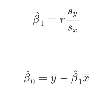{width=30% fig-align="center"}> where $r$ is the sample correlation between $y$ and $x$,$$r = \frac{\frac{1}{n}\sum_{i=1}^n(y_i - \bar{y})(x_i - \bar{x})}{\sqrt{\frac{1}{n}\sum_{i=1}^n(y_i-\bar{y})^2}\sqrt{\frac{1}{n}\sum_{i=1}^n(x_i-\bar{x})^2}},$$> and $s_x$ and $s_y$ are the sample standard deviation of $x$ and $y$, respectively: $$s_x = \sqrt{\frac{1}{n}\sum_{i=1}^n(x_i-\bar{x})^2}, s_y = \sqrt{\frac{1}{n}\sum_{i=1}^n(y_i-\bar{y})^2}.$$> Putting this together, the result from the Stat 155 Notes tells us that the slope coefficient estimate is $$\begin{aligned}\hat\beta_1 &= r \frac{s_y}{s_x} \\& = \left(\frac{\frac{1}{n}\sum_{i=1}^n(y_i - \bar{y})(x_i - \bar{x})}{\sqrt{\frac{1}{n}\sum_{i=1}^n(y_i-\bar{y})^2}\sqrt{\frac{1}{n}\sum_{i=1}^n(x_i-\bar{x})^2}}\right) \frac{\sqrt{\frac{1}{n}\sum_{i=1}^n(y_i-\bar{y})^2}}{\sqrt{\frac{1}{n}\sum_{i=1}^n(x_i-\bar{x})^2}} \\& = \frac{\frac{1}{n}\sum_{i=1}^n(y_i - \bar{y})(x_i - \bar{x})}{\frac{1}{n}\sum_{i=1}^n(x_i-\bar{x})^2} \\& = \frac{\sum_{i=1}^n(y_i - \bar{y})(x_i - \bar{x})}{\sum_{i=1}^n(x_i-\bar{x})^2}\end{aligned}$$> At first glance, this may not look the result we got above. > However, note that $\sum_{i=1}^n y_i x_i - n \bar{y}\bar{x} = \sum_{i=1}^n (y_i - \bar{y}) (x_i - \bar{x})$:$$\begin{aligned}\sum_{i=1}^n (y_i - \bar{y}) (x_i - \bar{x}) & = \sum_{i=1}^n (y_i x_i - y_i \bar{x} - \bar{y}x_i + \bar{y}\bar{x}) \\& = \sum_{i=1}^n y_i x_i - \sum_{i=1}^n y_i \bar{x} - \sum_{i=1}^n \bar{y} x_i + \sum_{i=1}^n \bar{y} \bar{x} \\& = \sum_{i=1}^n y_i x_i - \bar{x}\sum_{i=1}^n y_i - \bar{y}\sum_{i=1}^n x_i + n \bar{y} \bar{x} \\& = \sum_{i=1}^n y_i x_i - \bar{x}(n \bar{y}) - \bar{y}(n \bar{x}) + n \bar{y} \bar{x} \\& = \sum_{i=1}^n y_i x_i - n \bar{y}\bar{x}\end{aligned}$$> We can use a similar approach to show that $\sum_{i=1}^n x_i^2 - n \bar{x}^2 = \sum_{i=1}^n (x_i - \bar{x})^2$.## Part 6: Matrix Version of Least SquaresDeriving the least squares and maximum likelihood estimates for $\beta_0$ and $\beta_1$ was perhaps a bit tedious, but do-able, for a simple linear regression model with one explanatory variable. Things get more difficult when we consider multiple linear regression models with many explanatory variables:$$E[y | x_1, x_2, ..., x_p] = \beta_0 + \beta_1 x_1 + \beta_2 x_2 + \dots \beta_p x_p.$$When we have many explanatory variables, it's often useful to formulate our linear regression model using vectors and matrices. Consider the vector of outcomes $\mathbf{y}$$$\mathbf{y} = \begin{pmatrix} y_1 \\ y_2 \\ \vdots \\ y_n \end{pmatrix},$$the vector of covariates $\boldsymbol\beta$$$\boldsymbol\beta = \begin{pmatrix} \beta_0 \\ \beta_1 \\ \vdots \\ \beta_p \end{pmatrix},$$and the matrix of covariates (sometimes referred to as the "design matrix") $\mathbf{X}$$$\mathbf{X} = \begin{pmatrix} 1 & x_{11} & \cdots & x_{p1} \\ 1 & x_{12} & \cdots & x_{p2} \\ \vdots & \vdots & \ddots & \vdots \\ 1 & x_{1n} & \cdots & x_{pn} \end{pmatrix}.$$Then, we can write our linear regression model as $$E[\mathbf{y} \mid \mathbf{X}] = \mathbf{X} \boldsymbol\beta$$ or $$\mathbf{y} = \mathbf{X}\boldsymbol\beta + \boldsymbol\epsilon,$$ where $E[\boldsymbol\epsilon] = \mathbf{0}$.**Linear Algebra Review.** What are the dimensions of $\mathbf{X}$ and $\boldsymbol\beta$? What will be the dimension of their product $\mathbf{X} \boldsymbol\beta$?> $\mathbf{X}$ is a $n$-by-$(p + 1)$ matrix> > $\boldsymbol\beta$ is a vector of length $p + 1$, or a $(p + 1)$-by-1 matrix>> $\mathbf{X} \boldsymbol\beta$ will be an $n$-by-1 matrix**Linear Algebra Review (continued).** Calculate at least a few of the entries of $\mathbf{X} \boldsymbol\beta$ to confirm that this is an appropriate way to represent our linear regression model equation. $$\begin{aligned}\mathbf{X}\boldsymbol\beta & = \begin{pmatrix} 1 & x_{11} & \cdots & x_{p1} \\ 1 & x_{12} & \cdots & x_{p2} \\ \vdots & \vdots & \ddots & \vdots \\ 1 & x_{1n} & \cdots & x_{pn} \end{pmatrix} \begin{pmatrix} \beta_0 \\ \beta_1 \\ \vdots \\ \beta_p \end{pmatrix} \\& = \begin{pmatrix} 1 \times \beta_0 + x_{11}\times\beta_1 + \dots + x_{p1}\times\beta_p \\1 \times \beta_0 + x_{12}\times\beta_1 + \dots + x_{p2}\times\beta_p \\\vdots \\1 \times \beta_0 + x_{1n}\times\beta_1 + \dots + x_{pn}\times\beta_p \\\end{pmatrix} \\& = \begin{pmatrix} \beta_0 + \beta_1 x_{11} + \dots + \beta_p x_{p1} \\\beta_0 + \beta_1 x_{12} + \dots + \beta_p x_{p2} \\\vdots \\\beta_0 + \beta_1 x_{1n} + \dots + \beta_p x_{pn} \\\end{pmatrix} \\\end{aligned}$$> Notice that each entry in the resulting vector looks like what we are used to seeing in our model equation ($\beta_0 + \beta_1 x_{1i} + \dots + \beta_p x_{pi}$).Using matrix notation, we can now formulate the least squares problem as follows: $$\text{argmin}_{\boldsymbol\beta} (\mathbf{y} - \mathbf{X}\boldsymbol\beta)^\top(\mathbf{y} - \mathbf{X}\boldsymbol\beta),$$where the notation $\text{argmin}_{\boldsymbol\beta} f(\boldsymbol\beta)$ means that we want to find the value of $\boldsymbol\beta$ that minimizes the function $f(\boldsymbol\beta)$.**Linear Algebra Review (continued).** Convince yourself that the expression $(\mathbf{y} - \mathbf{X}\boldsymbol\beta)^\top(\mathbf{y} - \mathbf{X}\boldsymbol\beta)$ is equivalent to the sum of squared residuals $\sum_{i=1}^n r_i^2$ as we're used to seeing it. $$\begin{aligned}(\mathbf{y} - \mathbf{X}\boldsymbol\beta)^\top(\mathbf{y} - \mathbf{X}\boldsymbol\beta) & = \left(\begin{pmatrix} y_1 \\ \vdots \\ y_n \end{pmatrix} -\begin{pmatrix} \beta_0 + \beta_1 x_{11} + \dots + \beta_p x_{p1} \\\vdots \\\beta_0 + \beta_1 x_{1n} + \dots + \beta_p x_{pn} \\\end{pmatrix} \right)^\top \left(\begin{pmatrix} y_1 \\ \vdots \\ y_n \end{pmatrix} -\begin{pmatrix} \beta_0 + \beta_1 x_{11} + \dots + \beta_p x_{p1} \\\vdots \\\beta_0 + \beta_1 x_{1n} + \dots + \beta_p x_{pn} \\\end{pmatrix} \right) \\& = \begin{pmatrix} y_1 - (\beta_0 + \beta_1 x_{11} + \dots + \beta_p x_{p1}) \\\vdots \\y_n - (\beta_0 + \beta_1 x_{1n} + \dots + \beta_p x_{pn}) \\\end{pmatrix} ^\top \begin{pmatrix} y_1 - (\beta_0 + \beta_1 x_{11} + \dots + \beta_p x_{p1}) \\\vdots \\y_n - (\beta_0 + \beta_1 x_{1n} + \dots + \beta_p x_{pn}) \\\end{pmatrix} \\& = \begin{pmatrix} y_1 - (\beta_0 + \beta_1 x_{11} + \dots + \beta_p x_{p1}) &\cdots &y_n - (\beta_0 + \beta_1 x_{1n} + \dots + \beta_p x_{pn}) \\\end{pmatrix} \begin{pmatrix} y_1 - (\beta_0 + \beta_1 x_{11} + \dots + \beta_p x_{p1}) \\\vdots \\y_n - (\beta_0 + \beta_1 x_{1n} + \dots + \beta_p x_{pn}) \\\end{pmatrix} \\& = [y_1 - (\beta_0 + \beta_1 x_{11} + \dots + \beta_p x_{p1})] [y_1 - (\beta_0 + \beta_1 x_{11} + \dots + \beta_p x_{p1})] + \cdots + [y_n - (\beta_0 + \beta_1 x_{1n} + \dots + \beta_p x_{pn}) ] [y_n - (\beta_0 + \beta_1 x_{1n} + \dots + \beta_p x_{pn}) ]\\& = [y_1 - (\beta_0 + \beta_1 x_{11} + \dots + \beta_p x_{p1})]^2 + \cdots + [y_n - (\beta_0 + \beta_1 x_{1n} + \dots + \beta_p x_{pn}) ]^2 \\& = \sum_{i=1}^n [y_i - (\beta_0 + \beta_1 x_{1i} + \dots + \beta_p x_{pi})]^2 \end{aligned}$$## Part 7: Matrix CalculusOur next step is to find the value of $\boldsymbol\beta$ that minimizes the sum of squared residuals $(\mathbf{y} - \mathbf{X}\boldsymbol\beta)^\top(\mathbf{y} - \mathbf{X}\boldsymbol\beta)$.There are some useful results about [derivatives of vectors](http://www.gatsby.ucl.ac.uk/teaching/courses/sntn/sntn-2017/resources/Matrix_derivatives_cribsheet.pdf) and [matrices](https://drive.google.com/file/d/1SnpeNAP75ufBIgvfmb68PxLLP9mc-wyg/view?usp=sharing) that will be helpful for this derivation. In particular: - $(a + b)^\top c = a^\top c + b^\top c$- $(AB)^\top = B^\top A^\top$- $a^\top b = b^\top a$- $\frac{\partial}{\partial \mathbf{a}} \mathbf{a}^\top \mathbf{b} = \mathbf{b} = \frac{\partial}{\partial \mathbf{a}} \mathbf{b}^\top \mathbf{a}$- $\frac{\partial}{\partial \mathbf{a}} \mathbf{a}^\top \mathbf{B} \mathbf{a} = 2\mathbf{B}\mathbf{a}$:::{.callout-tip title="Challenge"}For this assignment, you can use these results without proof. But, it would be a useful exercise to confirm for yourself that all (or at least some) of these results are true!:::Using these results, find the derivative of the sum of squared residuals with respect to $\boldsymbol\beta$: $$\begin{aligned}\frac{\partial}{\partial \boldsymbol\beta} (\mathbf{y} - \mathbf{X}\boldsymbol\beta)^\top(\mathbf{y} - \mathbf{X}\boldsymbol\beta) & = \frac{\partial}{\partial \boldsymbol\beta} \left(\mathbf{y}^\top \mathbf{y} - (\mathbf{X}\boldsymbol\beta)^\top\mathbf{y} - \mathbf{y}^\top (\mathbf{X}\boldsymbol\beta) + (\mathbf{X}\boldsymbol\beta)^\top (\mathbf{X}\boldsymbol\beta) \right)\\& = \frac{\partial}{\partial \boldsymbol\beta} \left(\mathbf{y}^\top \mathbf{y} - 2\mathbf{y}^\top\mathbf{X}\boldsymbol\beta + \boldsymbol\beta^\top \mathbf{X}^\top \mathbf{X} \boldsymbol\beta \right) \\& = -2\mathbf{X}^\top\mathbf{y} + 2 \mathbf{X}^\top \mathbf{X} \boldsymbol\beta\end{aligned}$$Then, set this equal to zero and solve for $\boldsymbol\beta$:$$\begin{aligned}-2\mathbf{X}^\top\mathbf{y} + 2 \mathbf{X}^\top \mathbf{X} \boldsymbol\beta &\stackrel{set}{=} 0 \\2 \mathbf{X}^\top \mathbf{X} \boldsymbol\beta & = 2\mathbf{X}^\top\mathbf{y} \\\mathbf{X}^\top \mathbf{X} \boldsymbol\beta & = \mathbf{X}^\top\mathbf{y} \\(\mathbf{X}^\top \mathbf{X})^{-1}\mathbf{X}^\top \mathbf{X} \boldsymbol\beta & = (\mathbf{X}^\top \mathbf{X})^{-1}\mathbf{X}^\top\mathbf{y} \\\implies \hat{\boldsymbol\beta} & = (\mathbf{X}^\top \mathbf{X})^{-1}\mathbf{X}^\top\mathbf{y} \end{aligned}$$Check your answer: you should end up with the solution $\hat{\boldsymbol\beta} = (\mathbf{X}^\top \mathbf{X})^{-1}\mathbf{X}^\top\mathbf{y}$.:::{.callout-tip}Go one step further. Suppose we just have a single predictor variable, so $\mathbf{X} = \begin{bmatrix} 1 & x_{11} \\ 1 & x_{12} \\ & \vdots \\ 1 & x_{1n} \end{bmatrix}$. Calculate $(\mathbf{X}^\top \mathbf{X})^{-1}\mathbf{X}^\top\mathbf{y}$. Your result should be a 2-by-1 matrix, where the two entries match your $\hat\beta_0, \hat\beta_1$ from Part 5.:::## Part 8: The p > n problem, revisitedNow that we've done all that math, we can finally come back to our p > n problem. We saw above that the least squares estimator for the coefficients of a multiple linear regression model can be written as $$\hat{\boldsymbol\beta} = (\mathbf{X}^\top \mathbf{X})^{-1}\mathbf{X}^\top\mathbf{y}.$$Let's calculate $\mathbf{X}^\top \mathbf{X}$ for our toy example, above:```{r}xtx <-t(snps) %*% snps```What is the determinant of $\mathbf{X}^\top \mathbf{X}$?```{r calculate-determinant}det(xtx)```What does this tell us about $(\mathbf{X}^\top \mathbf{X})^{-1}$?> Since the determinant of $\mathbf{X}^\top \mathbf{X}$ is zero, this tell us that it is not invertible. In other words, $(\mathbf{X}^\top \mathbf{X})^{-1}$ does not exist, and thus our least squares estimator $$\hat{\boldsymbol\beta} = (\mathbf{X}^\top \mathbf{X})^{-1}\mathbf{X}^\top\mathbf{y}$$ is not defined.> Another way to think about this: since $\mathbf{X}$ has more columns than rows, the columns are not linearly independent and thus it is not full rank. What does this tell us about $\mathbf{X}^\top \mathbf{X}$? Review your notes from Linear Algebra if needed :)
