---
title: "Principal Component Regression (Notes)"
subtitle: "Stat 253"
author: "Your Name"
format:
html:
toc: true
toc-depth: 2
embed-resources: true
---
```{r include = FALSE}
knitr::opts_chunk$set(
collapse = TRUE,
warning = FALSE,
message = FALSE,
fig.height = 2.75,
fig.width = 4.25,
fig.env='figure',
fig.pos = 'h',
fig.align = 'center')
```
# Learning Goals {-}
- Explain the goal of dimension reduction and how this can be useful in a supervised learning setting
- Clearly describe / implement the principal component regression algorithm
- Describe the tradeoff of choice of principal components ($k$) in terms of the bias-variance tradeoff
- Implement strategies for choosing $k$
- Discuss the pros and cons of principal component regression relative to variable selection and LASSO
\
\
\
# Small Group Discussion {-}
Let's review some ideas from last class!
## Example 1 {-}
What is the goal of Principal Component Analysis?
## Example 2 {-}
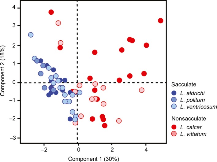
Consider the following PCA results from a paper written by Macalester faculty (Sarah Boyer, Biology; Dennis Cao, Chemistry) and student collaborators:
{width=80%}
a. What is this type of plot called?
b. If the authors want to retain at least 50% of the variance in the original features, how many/which PCs should they keep?
c. When describing this figure in [their paper](https://pmc.ncbi.nlm.nih.gov/articles/PMC6131725/), the authors say: "Principal components analysis (PCA) on the free amino acid profiles of the harvestmen specimens yielded four PCs with eigenvalues exceeding 1, which collectively explain 70.6% of the total variation in amino acid composition. PC1 explains 30.2% of the variation and is characterized by positive loading of alanine, valine, phenylalanine, glutamic acid, and tyrosine, and negative loading of isoleucine and threonine. PC2 accounts for a further 17.7% of the variation and is characterized by positive loading of ..."
- What is a *loading*?
- What is the connection between loadings and *scores*?
- What can we learn from loadings about the original features?
\
## Bonus {-}
Fun Fact: Professor Grinde's latest paper is also about PCA (and PC Regression)!
Check it out here if you're interested: [Adjusting for principal components can induce collider bias in genome-wide association studies](https://journals.plos.org/plosgenetics/article?id=10.1371/journal.pgen.1011242).
\
\
\
# Notes: PC Regression {-}
## Context {.unnumbered .smaller}
We've been distinguishing 2 broad areas in machine learning:
- supervised learning: when we want to predict / classify some outcome y using predictors x
- unsupervised learning: when we don't have any outcome variable y, only features x
- clustering: examine structure among the rows with respect to x
- dimension reduction: examine & combine structure among the columns x
BUT sometimes we can combine these ideas!
\
## Combining Forces {.unnumbered .smaller}
**Dimension Reduction + Clustering**
1. Use dimension reduction to visualize / summarize lots of features and notice interesting groups.
Example: many physical characteristics of penguins, many characteristics of songs, etc
2. Use clustering to identify interesting groups.
Example: types (species) of penguins, types (genres) of songs, etc
**Clustering + Classification**
1. Use clustering to identify interesting groups.
Example: types (species) of penguins, types (genres) of songs, etc
2. These groups might then become our $y$ outcome variable in future analysis.
Example: classify new penguins as one of the "species" we identified, classify new songs as one of the "genres" we identified
EXAMPLE: [K-means clustering + Classification of news articles](https://github.com/AustinKrause/nyt-article-summarizer)
\
## Dimension Reduction + Regression: Dealing with lots of predictors {.unnumbered .smaller}
Suppose we have an outcome variable $y$ (quantitative OR categorical) and lots of potential predictors $x_1, x_2, ..., x_p$.
Perhaps we even have more predictors than data points ($p > n$)!
This idea of measuring lots of things on a sample is common in genetics, image processing, video processing, or really any scenario where we can grab data on a bunch of different features at once.
For simplicity, computational efficiency, avoiding overfitting, etc, it might benefit us to simplify our set of predictors.
There are a few approaches:
- **variable selection (eg: using backward stepwise)**
Simply kick out some of the predictors.
NOTE: This doesn't work when $p > n$.
- **regularization (eg: using LASSO)**
Shrink the coefficients toward / to 0.
NOTE: This *sorta* works when $p > n$.
- **feature extraction (eg: using PCA)**
Identify & utilize only the most *salient* features of the original predictors.
Specifically, combine the original, possibly correlated predictors into a smaller set of uncorrelated predictors which retain most of the original information.
NOTE: This *does* work when $p > n$.
## Principal Component Regression (PCR) {.unnumbered .smaller}
- **Step 1**
Ignore $y$ for now.
Use PCA to combine the $p$ original, correlated predictors $x$ into a set of $p$ uncorrelated PCs.
- **Step 2**
Keep only the first $k$ PCs which retain a "sufficient" amount of information from the original predictors.
- **Step 3**
Model $y$ by these first $k$ PCs.
## PCR vs Partial Least Squares {.unnumbered .smaller}
When combining the original predictors $x$ into a smaller set of PCs, PCA *ignores* $y$. Thus PCA might not produce the strongest possible predictors of $y$.
**Partial least squares** provides an alternative.
Like PCA, it combines the original predictors into a smaller set of uncorrelated features, but considers which predictors are most associated with $y$ in the process.
Chapter 6.3.2 in ISLR provides an optional overview.
\
\
\
\
# Small Group Discussion {-}
## Example 3 {.unnumbered .smaller}
For each scenario below, indicate which would (typically) be preferable in modeling y by a large set of predictors x: (1) PCR; or (2) variable selection or regularization.
a. We have more potential predictors than data points ($p > n$).
b. It's important to understand the specific relationships between y and x.
c. The x are NOT very correlated.
\
\
\
# Exercises {-}
Use the rest of class time to work on HW7 and Group Assignment 3.
Decide **as a group** how you will split your time!
## HW7 {-}
Exercises 3 focuses on PC Regression.
In Exercise 4, you will compare your PC Regression model to LASSO.
Use the R Code Notes below to help with this!
Remember to `set.seed(253)` on any exercises that involve randomness.
## Group Assignment 3 {.unnumbered .smaller}
Before you leave class today:
1. Get data on your local computers
2. Start exploring the data:
- Familiarize yourself with the variables
- Create initial visualizations
- Determine if any data cleaning is needed (remove, modify, or create variables; remove or fill in missing values; remove observations)
3. Make a plan:
- How to decide which features to use, how many and which algorithms to try, how to evaluate each algorithm
- Set up communication avenues for out-of-class discussions (slack channel? in-person meetings? etc.)
- Divide / delegate leadership on tasks
\
\
\
# Notes: R Code {-}
Suppose we have a set of `sample_data` with multiple predictors x, a *quantitative* outcome y, and (possibly) a column named `data_id` which labels each data point.
We could adjust this code if y were *categorical*.
---------------------
**RUN THE PCR algorithm**
```{r eval = FALSE}
# load packages
library(tidymodels)
library(tidyverse)
# STEP 1: specify a linear regression model
lm_spec <- linear_reg() %>%
set_mode("regression") %>%
set_engine("lm")
# STEP 2: variable recipe
# Add a pre-processing step that does PCA on the predictors
# num_comp is the number of PCs to keep (we need to tune it!)
# remove the update_role line if you don't have an ID variable you want to ignore in your model/PCA
pcr_recipe <- recipe(y ~ ., data = sample_data) %>%
update_role(data_id, new_role = "id") %>%
step_dummy(all_nominal_predictors()) %>%
step_normalize(all_predictors()) %>%
step_pca(all_predictors(), num_comp = tune())
# STEP 3: workflow
pcr_workflow <- workflow() %>%
add_recipe(pcr_recipe) %>%
add_model(lm_spec)
# STEP 4: Estimate multiple PCR models trying out different numbers of PCs to keep
# For the range, the biggest number you can try is the number of predictors you started with
# Put the same number in levels
set.seed(___)
pcr_models <- pcr_workflow %>%
tune_grid(
grid = grid_regular(num_comp(range = c(1, ___)), levels = ___),
resamples = vfold_cv(sample_data, v = 10),
metrics = metric_set(mae)
)
```
\
**FOLLOW-UP**
Processing and applying the results is the same as for our other `tidymodels` algorithms!
Review previous notes to remind yourself how functions like `autoplot`, `select_by_one_std_err`, and `collect_metrics` work.
# Done!
- Render your notes.
- Check the solutions in the course website (Solution drop downs).
- If you finish all that during class, start your homework!