---
title: "Hierarchical Clustering (Notes)"
subtitle: "Stat 253"
author: "Your Name"
format:
html:
toc: true
toc-depth: 2
embed-resources: true
---
```{r include = FALSE}
knitr::opts_chunk$set(
collapse = TRUE,
warning = FALSE,
message = FALSE,
fig.height = 2.75,
fig.width = 4.25,
fig.env='figure',
fig.pos = 'h',
fig.align = 'center')
```
# Learning Goals {.unnumbered .smaller}
- Clearly describe / implement by hand the hierarchical clustering algorithm
- Interpret cuts of the dendrogram for single and complete linkage
- Implement strategies for interpreting / contextualizing the clusters
\
\
# Notes: Unsupervised Learning {-}
## Context {.unnumbered .smaller}
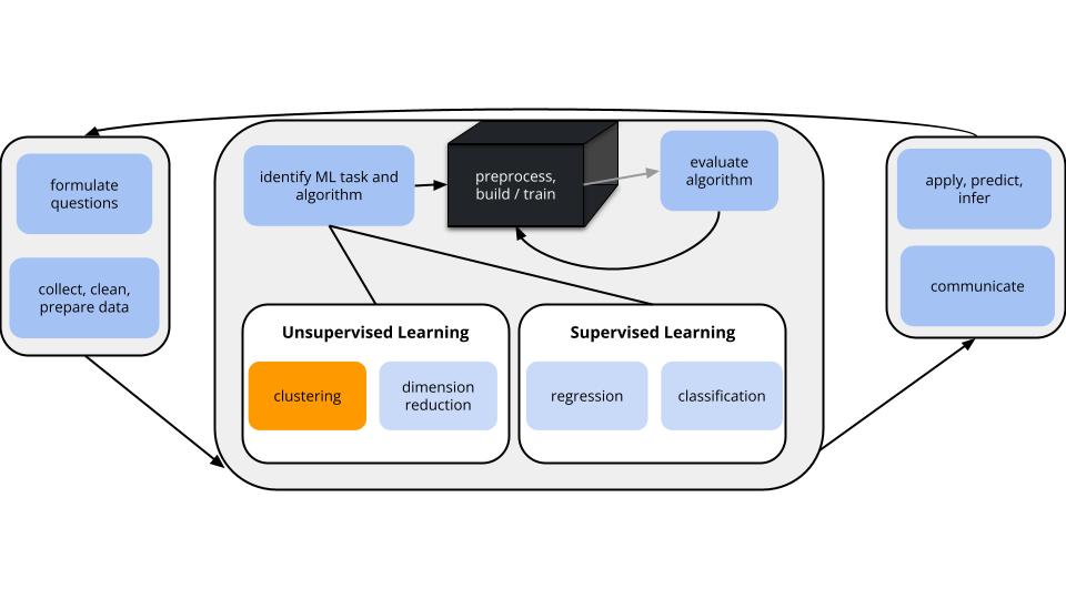{width=90%}
**GOALS**
Suppose we have a set of **feature** variables $(x_1,x_2,...,x_k)$ but NO outcome variable $y$.
Instead of our goal being to predict/classify/explain $y$, we might simply want to...
1. Examine the **structure** of our data.
2. Utilize this examination as a **jumping off point** for further analysis.
\
## Unsupervised Methods {.unnumbered .smaller}
Cluster Analysis (Unit 6):
- Focus: Structure among the *rows*, i.e. individual cases or data points.
- Goal: Identify and examine *clusters* or distinct groups of cases with respect to their features x.
- Methods: hierarchical clustering & K-means clustering
Dimension Reduction (Unit 7):
- Focus: Structure among the *columns*, i.e. features x.
- Goal: *Combine* groups of correlated features x into a smaller set of *uncorrelated* features which preserve the majority of information in the data. (We'll discuss the motivation later!)
- Methods: Principal components
\
## Examples {.unnumbered .smaller}
Remember this from the first day of class?
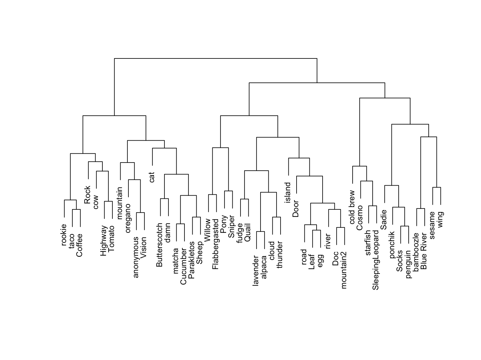{width=90%}
For more examples, check out the Unit 6 Motivating Question page [here](U06-motivation.html).
# Notes: Hierarchical Cluster Analysis {-}
Let's recap the main ideas from the videos you watched before class today.
\
## Goal {.unnumbered .smaller}
Create a hierarchy of clusters where clusters consist of similar data points.
\
## Algorithm {.unnumbered .smaller}
Suppose we have a set of p feature variables ($x_1, x_2,..., x_p$) on each of n data points. Each data point starts as a leaf.
- Compute the Euclidean distance between all pairs of data points with respect to x.
- Fuse the 2 closest data points into a single cluster or branch.
- Continue to fuse the 2 closest clusters until all cases are in 1 cluster.
NOTE: This is referred to as an "agglomerative" algorithm.
\
## Dendrograms {.unnumbered .smaller}
The hierarchical clustering algorithm produces a *dendrogram* (of or relating to trees).
To use a dendrogram:
:::{.incremental}
- Start with the leaves at the bottom (unlike classification trees!). Each leaf represents a single case / row in our dataset.
- Moving up the tree, fuse similar leaves into branches, fuse similar branches into bigger branches, fuse all branches into one big trunk (all cases).
- The more similar two cases, the sooner their branches will fuse. The height of the first fusion between two cases’ branches measures the "distance" between them.
- The horizontal distance between 2 leaves does not reflect distance!
:::
\
## Measuring Distance {.unnumbered .smaller}
There are several *linkages* we can use to measure distance between 2 clusters / branches. Unless specified otherwise, we'll use the **complete** linkage method.
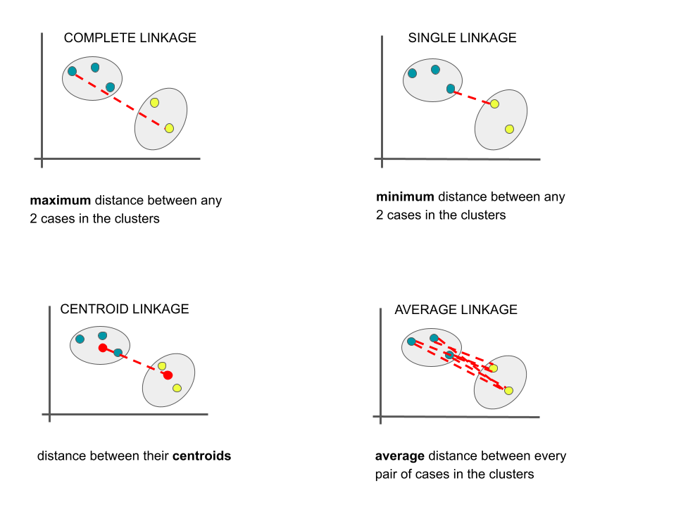
# Small Group Discussion {-}
## Example 1: Standardizing the features {.unnumbered .smaller}
Let's start by using hierarchical clustering to identify similar groups (and possible species!) of penguins with respect to their bill lengths (mm), bill depths (mm), and body masses (g).
This algorithm relies on calculating the distances between each pair of penguins.
Why is it important to first *standardize* our 3 features to the same scale (centered around a mean of 0 with standard deviation 1)?
```{r}
library(tidyverse)
library(palmerpenguins)
data("penguins")
penguins %>%
select(bill_length_mm, bill_depth_mm, body_mass_g) %>%
head()
```
\
## Example 2: Interpreting a dendrogram {.unnumbered .smaller}
Check out the standardized data, heat map, and dendrogram for a sample of just 50 penguins.
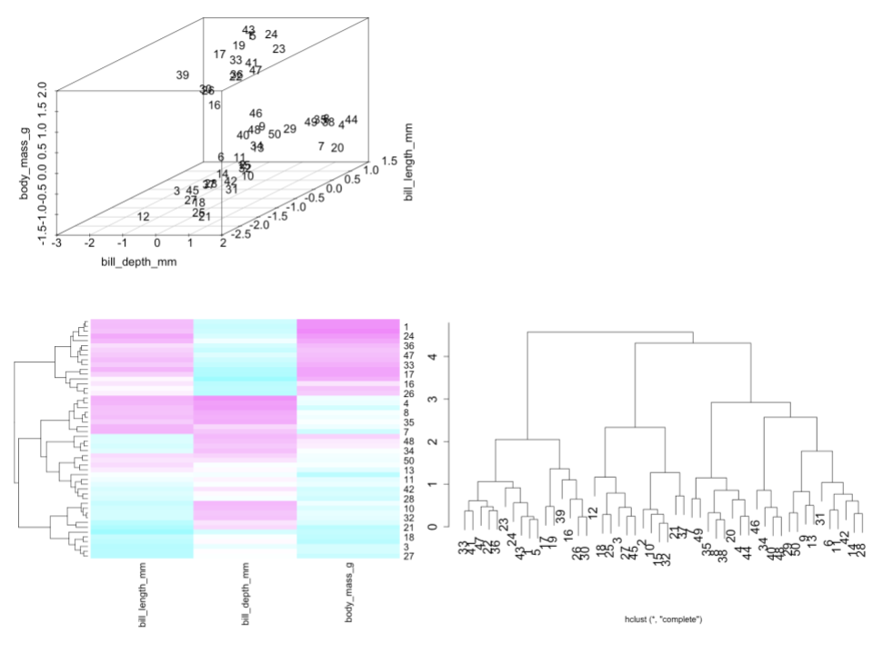
a. Is penguin 30 more similar to penguin 33 or 12?
b. Identify and interpret the distance, calculated using the *complete* linkage, between penguins 30 and 33.
c. Consider the far left penguin cluster on the dendrogram, starting with penguin 33 and ending with penguin 30. Use the heat map to describe what these penguins have in common.
\
## Example 3: By Hand {.unnumbered .smaller}
To really get the details, you'll perform hierarchical clustering by hand for a small example.
Ask you instructor for a copy of the [paper handout](https://docs.google.com/document/d/1abptMI_GsEM-LbGAFBRHRFsW8yJC9iajzjAqjxaCgpg/edit?usp=sharing).
Code for importing the data is here:
```{r}
#| fig-width: 4
#| fig-height: 4
#| eval: true
# Record the data
penguins_small <- data.frame(
width = c(-1.3, -0.8, 0.2, 0.8, 1.0),
length = c(0.6, 1.4, -1.0, -0.2, -0.7))
# Plot the data
ggplot(penguins_small, aes(x = width, y = length)) +
geom_point() +
geom_text(aes(label = c(1:5)), vjust = 1.5) +
theme_minimal()
# Calculate the distance between each pair of penguins
round(dist(penguins_small), 2)
# Type out the R code from Part b below
```
\
## Example 4: Explore Clusters {.unnumbered .smaller}
Now, let's go back to a sample of 50 penguins.
Run the 2 chunks below to build a shiny app that we'll use to build some intuition for hierarchical clustering.
a. Put the slider at 9 clusters. These 9 clusters are represented in the dendrogram and scatterplot of the data. Do you think that 9 clusters is too many, too few, or just right?
b. Now set the slider to 5. Simply take note of how the clusters appear in the data.
c. Now sloooooowly set the slider to 4, then 3, then 2. Each time, notice what happens to the clusters in the data plot. Describe what you observe.
d. What are your thoughts about the 2-cluster solution? What happened?!
```{r}
#| code-fold: true
# Load the data
library(tidyverse)
set.seed(253)
more_penguins <- penguins %>%
sample_n(50) %>%
select(bill_length_mm, bill_depth_mm) %>%
na.omit()
# Run hierarchical clustering
penguin_cluster <- hclust(dist(scale(more_penguins)), method = "complete")
# Record cluster assignments
clusters <- more_penguins %>%
mutate(k = rep(1, nrow(more_penguins)), cluster = rep(1, nrow(more_penguins)))
for(i in 2:12){
clusters <- more_penguins %>%
mutate(k = rep(i, nrow(more_penguins)),
cluster = cutree(penguin_cluster, k = i)) %>%
bind_rows(clusters)
}
```
```{r}
#| eval: false
#| code-fold: true
library(shiny)
library(factoextra)
library(RColorBrewer)
# Build the shiny server
server_hc <- function(input, output) {
dend_plot <- reactive({
cols = brewer.pal(n= input$k_pick, "Set1")
fviz_dend(penguin_cluster, k = input$k_pick, k_colors = cols)
})
output$model_plot <- renderPlot({
cols = brewer.pal(n= input$k_pick, "Set1")
dend <- attributes(dend_plot())$dendrogram
tree_order <- order.dendrogram(dend)
clusters_k <- clusters %>%
filter(k == input$k_pick)
clusters_k <- clusters_k %>%
mutate(cluster = factor(cluster, levels = unique(clusters_k$cluster[tree_order])))
names(cols) = unique(clusters_k$cluster[tree_order])
clusters_k %>%
ggplot(aes(x = bill_length_mm, y = bill_depth_mm, color = factor(cluster))) +
geom_point(size = 3) +
scale_color_manual(values = cols) +
theme_minimal() +
theme(legend.position = "none")
})
output$dendrogram <- renderPlot({
dend_plot()
})
}
# Build the shiny user interface
ui_hc <- fluidPage(
sidebarLayout(
sidebarPanel(
h4("Pick the number of clusters:"),
sliderInput("k_pick", "cluster number", min = 1, max = 9, value = 9, step = 1, round = TRUE)
),
mainPanel(
plotOutput("dendrogram"),
plotOutput("model_plot")
)
)
)
# Run the shiny app!
shinyApp(ui = ui_hc, server = server_hc)
```
\
## Example 5: Details {.unnumbered .smaller}
a. Is hierarchical clustering **greedy**?
b. We learned in the video that, though they both produce tree-like output, the hierarchical clustering and classification tree algorithms are *not the same thing*! Similarly, though they both calculate distances between each pair of data points, the hierarchical clustering and KNN algorithms are *not the same thing*! Explain.
Note: When all features x are quantitative or logical (TRUE/FALSE), we measure the similarity of 2 data points with respect to the Euclidean distance between their *standardized* x values. But if at least 1 feature x is a factor / categorical variable, we measure the similarity of 2 data points with respect to their Gower distance. The idea is similar to what we did in KNN (converting categorical x variables to dummies, and then standardizing), but the details are different.
If you're interested:
```{r eval = FALSE}
library(cluster)
?daisy
```
\
\
# Exercises {-}
For the rest of class, work together on HW6 Exercises 1--3.
We'll cover material in the next class to complete the rest of the exercises.
\
\
# Notes: R code {.unnumbered .smaller}
The `tidymodels` package is built for *models* of some outcome variable y.
We can't use it for clustering.
Instead, we'll use a variety of new packages that use specialized, but short, syntax.
---------------------
Suppose we have a set of `sample_data` with multiple feature columns x, and (possibly) a column named `id` which labels each data point.
```{r eval = FALSE}
# Install packages
library(tidyverse)
library(cluster) # to build the hierarchical clustering algorithm
library(factoextra) # to draw the dendrograms
```
\
**PROCESS THE DATA**
If there's a column that's an identifying variable or label, not a feature of the data points, convert it to a row name.
```{r eval = FALSE}
sample_data <- sample_data %>%
column_to_rownames("id")
```
\
**RUN THE CLUSTERING ALGORITHM**
```{r eval = FALSE}
# Scenario 1: ALL features x are quantitative OR logical (TRUE/FALSE)
# Use either a "complete", "single", "average", or "centroid" linkage_method
hier_model <- hclust(dist(scale(sample_data)), method = ___)
# Scenario 2: AT LEAST 1 feature x is a FACTOR (categorical)
# Use either a "complete", "single", "average", or "centroid" linkage
hier_model <- hclust(daisy(sample_data, metric = "gower"), method = ___)
```
\
**VISUALIZING THE CLUSTERING: HEAT MAPS AND DENDRODGRAMS**
NOTE: Heat maps can be goofy if at least 1 x feature is categorical
```{r eval = FALSE}
# Heat maps: ordered by the id variable (not clustering)
heatmap(scale(data.matrix(sample_data)), Colv = NA, Rowv = NA)
# Heat maps: ordered by dendrogram / clustering
heatmap(scale(data.matrix(sample_data)), Colv = NA)
# Dendrogram (change font size w/ cex)
fviz_dend(hier_model, cex = 1)
fviz_dend(hier_model, horiz = TRUE, cex = 1) # Plot the dendrogram horizontally to read longer labels
```
\
**DEFINING & PLOTTING CLUSTER ASSIGNMENTS**
```{r eval = FALSE}
# Assign each sample case to a cluster
# You specify the number of clusters, k
# We typically want to store this in a new dataset so that the cluster assignments aren't
# accidentally used as features in a later analysis!
cluster_data <- sample_data %>%
mutate(hier_cluster_k = as.factor(cutree(hier_model, k = ___)))
# Visualize the clusters on the dendrogram (change font size w/ cex)
fviz_dend(hier_model, k = ___, cex = 1)
fviz_dend(hier_model, k = ___, horiz = TRUE, cex = 1) # Plot the dendrogram horizontally to read longer labels
```
# Done!
- Render your notes.
- Check the solutions in the course website (Solution drop downs).
- If you finish all that during class, start your homework!