---
title: "LOESS and Splines (Notes)"
subtitle: "Stat 253"
author: "Your Name"
format:
html:
toc: true
toc-depth: 2
embed-resources: true
---
```{r include = FALSE}
knitr::opts_chunk$set(
collapse = TRUE,
warning = FALSE,
message = FALSE,
fig.height = 2.75,
fig.width = 4.25,
fig.env='figure',
fig.pos = 'h',
fig.align = 'center')
```
# Learning Goals {.unnumbered .smaller}
- Clearly describe the local regression algorithm for making a prediction
- Explain how bandwidth (span) relate to the bias-variance tradeoff
- Explain the advantages of splines over global transformations and other types of piecewise polynomials
- Explain how splines are constructed by drawing connections to variable transformations and least squares
- Explain how the number of knots relates to the bias-variance tradeoff
\
\
# Context {.unnumbered .smaller}
{width=100%}
------------------
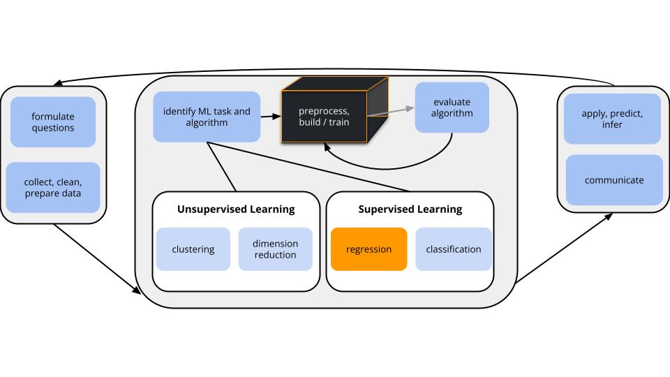
- **world = supervised learning**
We want to model some output variable $y$ using a set of potential predictors ($x_1, x_2, ..., x_p$) and the relationship could be non-linear.
- **task = regression**
$y$ is quantitative
- **a flexible algorithm**
Our standard *parametric* models (eg: linear regression) may too rigid to represent the relationship between $y$ and our predictors $x$. Thus we need more *flexible* **models**.
\
\
# KNN (Review) {-}
Discuss the following questions with your group to review key concepts from recent activities.
\
## Small Group Discussion {-}
1. **KNN Review**
In the previous activity, we modeled college `Grad.Rate` versus `Expend`, `Enroll`, and `Private` using data on 775 schools.
a. Which pre-processing steps are necessary for KNN, and why? How do we implement these pre-processing steps in R?
b. We chose the KNN with K = 33 because it *minimized* the CV MAE, i.e. the errors when predicting grad rate for schools *outside* our sample. We don't typically worry about a more *parsimonious* KNN, i.e. a model that has slightly higher prediction errors but is easier to interpret, apply, etc. Why?
c. What *assumptions* did the KNN model make about the relationship of `Grad.Rate` with `Expend`, `Enroll`, and `Private`? Is this a pro or con?
d. What did the KNN model tell us about the *relationship* of `Grad.Rate` with `Expend`, `Enroll`, and `Private`? For example, did it give you a sense of whether grad rates are higher at private or public institutions? At institutions with higher or lower enrollments? Is this a pro or con?
\
2. **Nonparametric vs Parametric**
Nonparametric KNN vs parametric least squares and LASSO:
- When *should* we use a nonparametric algorithm like KNN?
- When *shouldn't* we?
\
\
# LOESS {-}
## Notes {.unnumbered .smaller}
LOESS: _Local Regression_ or _**L**ocally **E**stimated **S**catterplot **S**moothing_
\
**Goal:**
Build a **flexible** regression model of $y$ by *one* quantitative predictor $x$,
$$y = f(x) + \varepsilon$$
\
**Idea:**
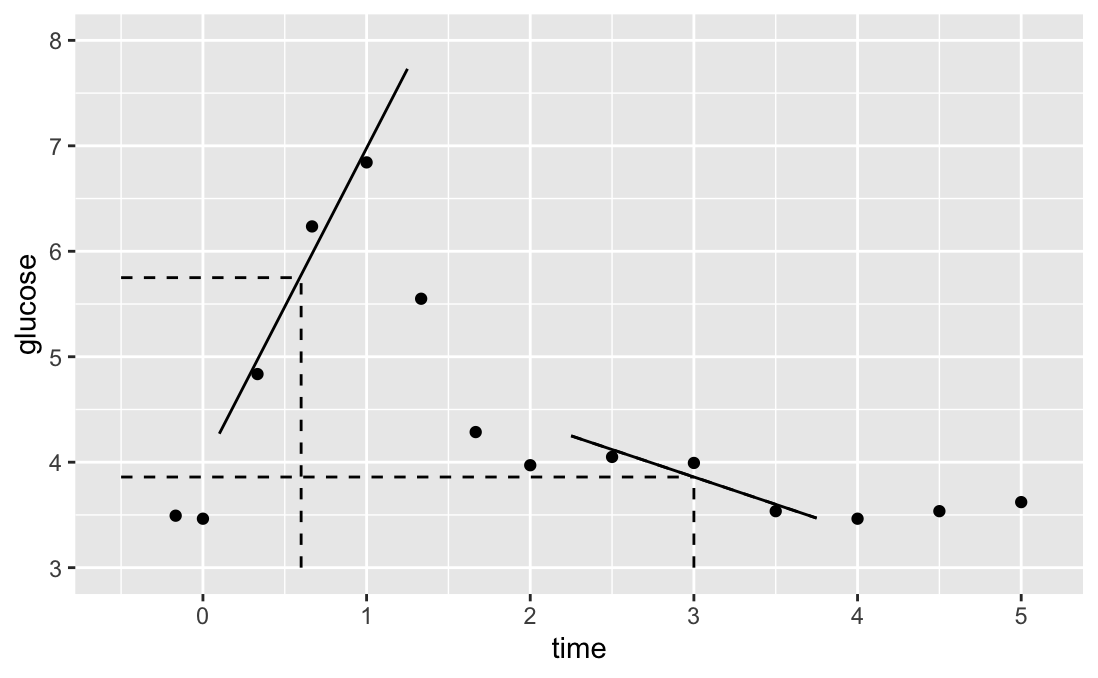
Fit regression models in small localized regions, where nearby data have greater influence than far data.
\
**Algorithm:**
Define the *span*, aka bandwidth, tuning parameter $h$ where $0 \le h \le 1$. Take the following steps to estimate $f(x)$ at each possible predictor value $x$:
1. Identify a neighborhood consisting of the $100∗h$% of cases that are closest to $x$.
2. Putting more weight on the neighbors closest to $x$ (ie. allowing them to have more influence), fit a linear model in this neighborhood.
3. Use the local linear model to estimate f(x).
\
**In pictures:**
{width=100%}
```{r loess-example}
#| eval: true
#| code-fold: true
library(tidyverse)
# example data
plot_data <- read.csv("https://bcheggeseth.github.io/253_spring_2024/data/glucose_experiment.csv")
# plot with LOESS predictions
plot_data %>%
ggplot() +
geom_point(aes(x = time, y = glucose)) +
geom_smooth(aes(x = time, y = glucose), se=FALSE) # this step does LOESS
```
\
\
## Small Group Discussion {.unnumbered .smaller}
Open the QMD and find the LOESS discussion questions.
Work on the following questions with your group.
\
3. **LOESS in R**
We can plot LOESS models using `geom_smooth()`. Play around with the `span` parameter below.
- What happens as we increase the span from roughly 0 to roughly 1?
- What is one "pro" of this nonparametric algorithm, relative to KNN?
- What questions do you have about this algorithm?
```{r loess-span}
#| eval: true
library(tidyverse)
library(ISLR)
data(College)
ggplot(College, aes(x = Expend, y = Grad.Rate)) +
geom_point() +
geom_smooth(method = "loess", span = 0.5)
```
Note: you'll find that you can specify `span` greater than 1.
Use your resources to figure out what that means in terms of the algorithm.
\
4. **LOESS & the Bias-Variance Tradeoff**
Run the **shiny app** code, below. Explore the impact of the *span tuning parameter h* on the LOESS performance across different datasets. Continue to click the Go! button to get different datasets.
For what values of $h$ (near 0, somewhere in the middle, near 1) do you get the following:
a. *high bias* but *low variance*
b. *low bias* but *high variance*
c. *moderate bias* and *low variance*
```{r loess-shiny}
#| eval: false
#| code-fold: true
# Load packages & data
library(shiny)
library(tidyverse)
# Define a LOESS plotting function
plot_loess <- function(h, plot_data){
ggplot(plot_data, aes(x = x, y = y)) +
geom_point() +
geom_smooth(span = h, se = FALSE) +
labs(title = paste("h = ", h)) +
lims(y = c(-5,12))
}
# BUILD THE SERVER
# These are instructions for building the app - what plot to make, what quantities to calculate, etc
server_LOESS <- function(input, output) {
new_data <- eventReactive(input$do, {
x <- c(runif(25, -6, -2.5), runif(50, -3, 3), runif(25, 2.5, 6))
y <- 9 - x^2 + rnorm(100, sd = 0.75)
y[c(1:25, 76:100)] <- rnorm(50, sd = 0.75)
data.frame(x, y)
})
output$loesspic <- renderPlot({
plot_loess(h = input$hTune, plot_data = new_data())
})
}
# BUILD THE USER INTERFACE (UI)
# The UI controls the layout, appearance, and widgets (eg: slide bars).
ui_LOESS <- fluidPage(
sidebarLayout(
sidebarPanel(
h4("Sample 100 observations:"),
actionButton("do", "Go!"),
h4("Tune the LOESS:"),
sliderInput("hTune", "h", min = 0.05, max = 1, value = 0.05)
),
mainPanel(
h4("LOESS plot:"),
plotOutput("loesspic")
)
)
)
# RUN THE SHINY APP!
shinyApp(ui = ui_LOESS, server = server_LOESS)
```
\
\
# Splines {-}
## Notes {.unnumbered .smaller}
**Goal:**
Build a **flexible** _parametric_ regression model of $y$ by one quantitative predictor $x$,
$$y = f(x) + \varepsilon$$
\
**Idea:**
Fit polynomial models in small localized regions and constrain to make it smooth enough.
\
**Definition:**
A spline is a piecewise polynomial of degree $k$ that is a continuous function and has continuous derivatives (of orders $1,...,k-1$) at its knot points (break points).
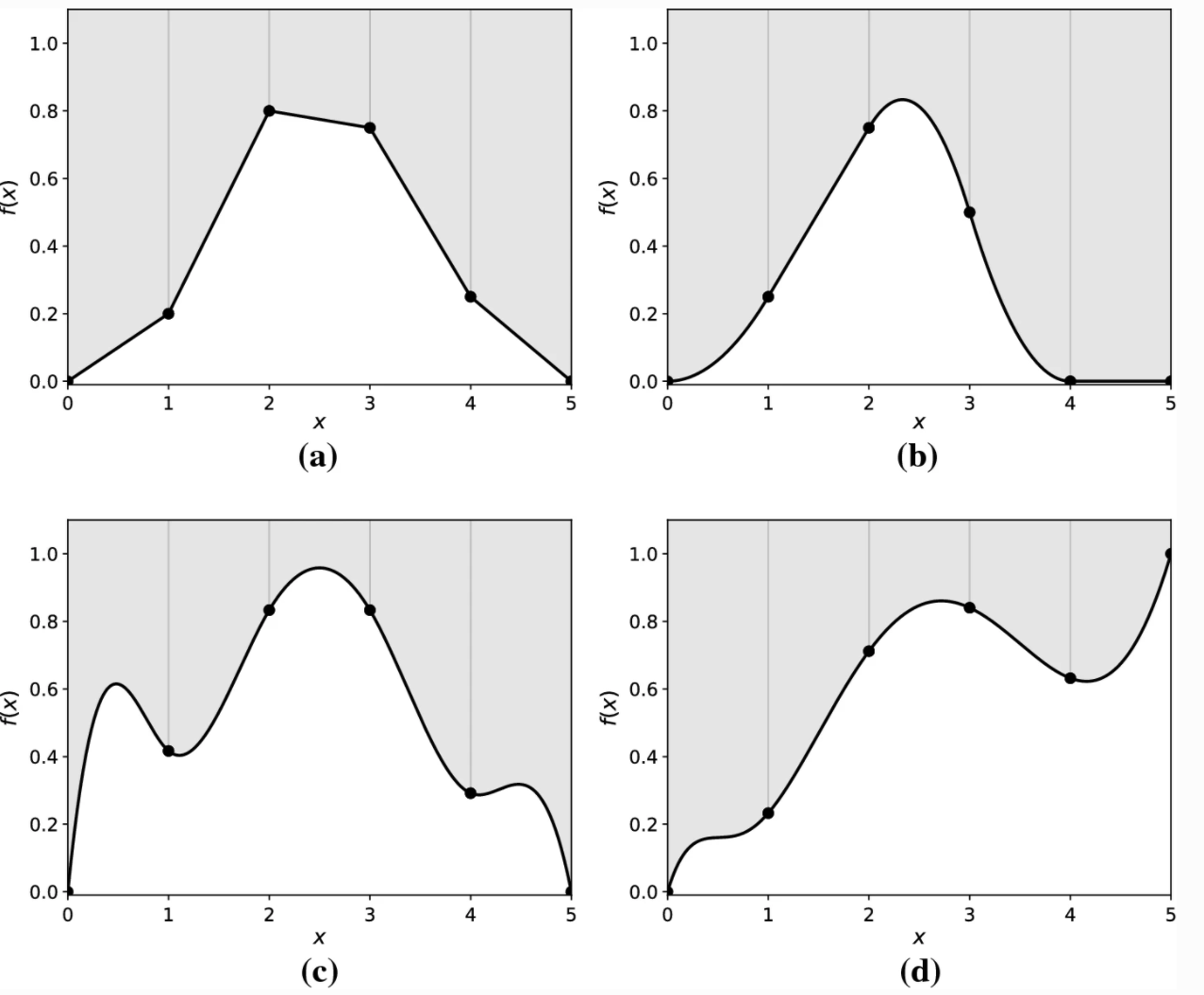 [Image source](https://link.springer.com/article/10.1007/s10898-020-00881-4)
A spline function $f$ with knot points $t_1<...
 [Image source](http://dx.doi.org/10.1038/s41598-023-49360-2)
Check out Section 7.4 in [ISLR](https://www.statlearning.com/) for more details!
\
\
## R Code {.unnumbered .smaller}
**Piecewise Polynomials in Stat 155**
If you had a quadratic model (degree = 2) with 0 knots, how could you fit that model using the tools of STAT 155?
```{r}
#| eval: false
lm(y ~ x + x2, data) #if you created x2 = x^2
lm(y ~ poly(x, 2), data)
```
If you had a piecewise linear model (degree = 1) with 1 knot at $x=5$, how could you fit that using the tools from Stat 155?
```{r}
#| eval: false
lm(y ~ x * I(x > 5), data)
```
These implementation methods don't constrain them to be continuous or smooth, so we need additional tools from the `splines` package!
\
**Splines in tidymodels**
To build models with splines in `tidymodels`, we proceed with the same structure as we use for ordinary linear regression models but we'll add some **pre-processing steps** to our `recipe`.
To work with splines, we'll use tools from the `splines` package in conjunction with `recipes`.
- The `step_ns()` function based on `ns()` in that package creates the transformations needed to create a natural cubic spline function for a quantitative predictor.
- The `step_bs()` function based on `bs()` in that package creates the transformations needed to create a basis spline (typically called B-splines) function for a quantitative predictor.
```{r splines-tidymodels}
#| eval: false
# Linear Regression Model Spec
lm_spec <-
linear_reg() %>%
set_mode('regression') %>%
set_engine(engine = 'lm')
# Original Recipe
lm_recipe <- recipe(y ~ x, data = sample_data)
# Polynomial Recipe
poly_recipe <- lm_recipe %>%
step_poly(x, degree = __) # polynomial (higher degree means more flexible)
# Natural Spline Recipe
ns2_recipe <- lm_recipe %>%
step_ns(x, deg_free = __) # natural cubic spline (higher deg_free means more knots)
# Basis Spline Recipe
bs_recipe <- lm_recipe %>%
step_bs(x, options = list(knots = c(__,__))) # b-spline (cubic by default, more knots means higher deg_free)
```
- The `deg_free` argument in `step_ns()` stands for degrees of freedom:
- `deg_free = # of knots + 1`
- The degrees of freedom are the number of coefficients in the transformation functions that are free to vary (essentially the number of underlying parameters behind the transformations).
- The knots are chosen using percentiles of the observed values.
- The `options` argument in `step_bs()` allows you to specific specific knots:
- `options = list(knots = c(2, 4))` sets a knot at 2 and a knot at 4 (the choice of knots should depend on the observed range of the quantitative predictor and where you see a change in the relationship)
\
**What is the difference between natural splines and B-splines?**
- B-spline is a tool to incorporate splines into a linear regression setting.
- You have to choose the knots (which can be tricky sometimes).
- These functions can be unstable (high variance) near the boundaries, especially with higher polynomial degrees.
- Natural spline is a variant of the B-spline with additional constraints on the boundaries to reduce variance (the degree of the polynomial near the boundaries is lower).
- Cubic natural splines are the most common
- Typically knots are chosen based on quantiles of the predictor (e.g. 1 knot will be placed at the median, 2 knots will be placed at the 33rd and 66th percentiles, etc.)
\
\
## Small Group Discussion {.unnumbered .smaller}
5. **Splines & the Bias-Variance Tradeoff**
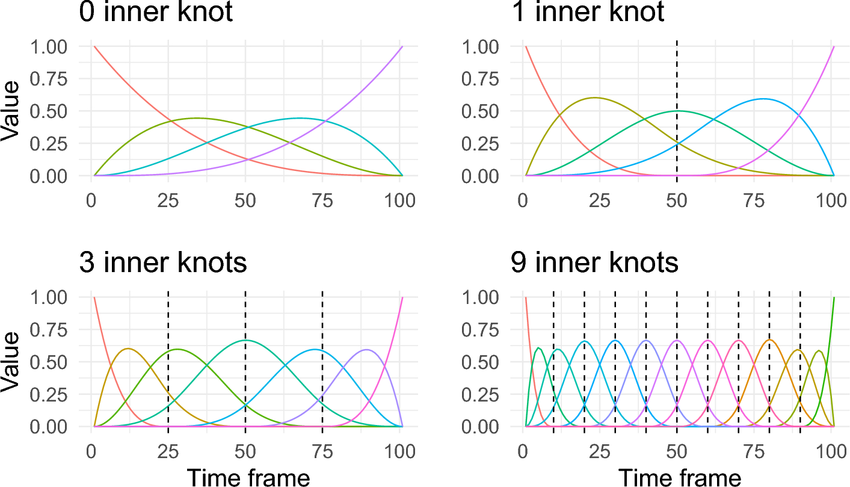
See the figure below, for either natural splines or cubic splines, what values of `deg_free` (small, medium, large) do you get the following:
a. *high bias* but *low variance*:
b. *low bias* but *high variance*:
c. *moderate bias* and *low variance*:
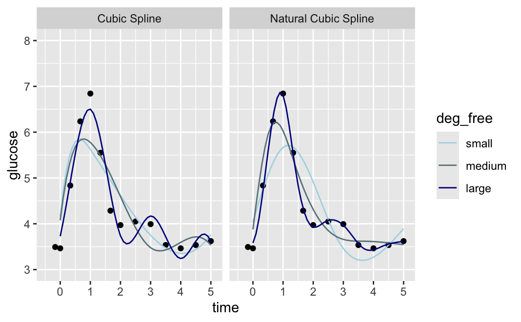
\
6. **splines & LASSO**
Could we use LASSO with a spline or polynomial recipe? Yes or No? Explain.
\
\
# Exercises {-}
## Part 1: Implementing Splines {.unnumbered .smaller}
**Goals**
- Implement and explore splines in R.
- Explore how this algorithm compares to others, hence how it fits into our broader ML workflow.
**Context**
Using the `College` data in the `ISLR` package, we'll build a predictive model of `Grad.Rate` by 6 predictors: `Private`, `PhD` (percent of faculty with PhDs), `Room.Board`, `Personal` (estimated personal spending), `Outstate` (out-of-state tuition), `perc.alumni` (percent of alumni who donate)
Before proceeding, install the `splines` package by entering `install.packages("splines")` in the Console.
```{r}
#| echo: true
#| eval: true
# Load packages
library(tidymodels)
library(tidyverse)
library(ISLR)
# Load data
data(College)
# Wrangle the data
college_sub <- College %>%
filter(Grad.Rate <= 100) %>%
filter((Grad.Rate > 50 | Expend < 40000)) %>%
select(Grad.Rate, Private, PhD, Room.Board, Personal, Outstate, perc.alumni)
```
\
\
1. **Evaluating a fully linear model**
We will model `Grad.Rate` as a function of the 6 predictors in `college_sub`.
a. Make scatterplots of each of the quantitative predictors and the outcome with 2 different smoothing lines to explore potential nonlinearity. Adapt the following code to create a scatterplot with a smooth LOESS blue trend line and a red linear trend line.
What do you notice about the form of the relationships?
```{r}
#| eval: false
ggplot(___, aes(___)) +
geom_point() +
geom_smooth(color = "blue", se = FALSE) +
geom_smooth(method = "lm", color = "red", se = FALSE) +
theme_classic()
```
```{r}
```
b. Use `tidymodels` to fit a linear regression model (no splines yet) with the following specifications:
- Use 8-fold CV.
- Use CV mean absolute error (MAE) to evaluate models.
- Use LASSO engine to do variable selection to select the simplest model for which the metric is within one standard error of the best metric.
- Fit your "best" model and look at coefficients of that final model. Which variables are "least" important to predicting `Grad.Rate`?
```{r}
#| eval: false
set.seed(253)
# Lasso Model Spec with tune
lasso_spec <- linear_reg() %>%
set_mode('regression') %>%
set_engine(engine = 'glmnet') %>%
set_args(mixture = 1, penalty = tune())
# Recipe
lasso_recipe <- recipe(__ ~ ___, data = college_sub) %>%
step_dummy(all_nominal_predictors())
# Workflow (Recipe + Model)
lasso_wf_tune <- workflow() %>%
add_recipe(lasso_recipe) %>%
add_model(lasso_spec)
# Tune Model (trying a variety of values of Lambda penalty)
lasso_models <- tune_grid(
lasso_wf_tune, # workflow
resamples = vfold_cv(__, v = __),
metrics = metric_set(___),
grid = grid_regular(penalty(range = c(-3, 1)), levels = 30)
)
# Select parsimonious model & fit
parsimonious_penalty <- lasso_models %>%
select_by_one_std_err(metric = 'mae', desc(penalty))
# Finalize Model
ls_mod <- lasso_wf_tune %>%
finalize_workflow(parameters = parsimonious_penalty) %>%
fit(data = college_sub)
# Note which variable is the "least" important
ls_mod %>%
tidy()
```
```{r}
```
c. Make a plot of the residuals vs. fitted values from` ls_mod` and then plots of the residuals v. each of the quantitative predictors to evaluate whether the model is "right".
```{r}
#| eval: false
ls_mod %>%
augment(new_data = college_sub) %>%
mutate(.resid = Grad.Rate - .pred) %>%
ggplot(aes(__)) +
___ +
geom_smooth(se = FALSE) +
geom_hline(yintercept = 0, color = "red") +
theme_classic()
```
```{r}
```
\
2. **Evaluating a spline model**
We'll compare our best LASSO model with models with spline functions for some of the quantitative predictors.
a. Update your recipe from Exercise 1 to fit a linear model (with the `lm` engine rather than `glmnet`) with the all predictors. Allow the quantitative predictors that had some non-linear relationships to be modeled with natural splines that have 4 degrees of freedom. Fit this model with 8 fold CV, `fit_resamples` (same folds as before) to compare MAE and then fit the model to the whole training data. Call this fit model `ns_mod`.
```{r}
#| eval: false
# Model Spec
lm_spec <-
linear_reg() %>%
set_mode('regression') %>%
set_engine(engine = 'lm')
# New Recipe (remove steps needed for LASSO, add splines)
# Create Workflow (Recipe + Model)
set.seed(253)
# CV to Evaluate
ns_models <- fit_resamples(
___, # workflow
resamples = vfold_cv(__, v = 8), # cv folds
metrics = metric_set(___)
)
ns_models %>% collect_metrics()
# Fit with all data
ns_mod <- fit( ___, #workflow from above
data = college_sub
)
```
```{r}
```
b. Make a plot of the residuals vs. fitted values from` ns_mod` and then plots of the residuals v. each of the quantitative predictors to evaluate whether the model is right.
```{r}
# Residual plots
```
c. Compare the CV MAE between models with and without the splines.
```{r}
#| error: true
lasso_models %>%
collect_metrics() %>%
filter(penalty == (parsimonious_penalty %>% pull(penalty)))
ns_models %>%
collect_metrics()
```
\
3. **Pick an algorithm**
Our overall goal is to build a predictive model of `Grad.Rate` ($y$) by 6 predictors:
$$y = f(x_1,x_2,...,x_{6}) + \varepsilon$$
The table below summarizes the CV MAE for 3 possible algorithms: least squares, KNN, and splines. After examining the results, explain which model you would choose and *why*. NOTE: There are no typos here! All models had virtually the same CV MAE. Code is provided in the online manual if you're curious.
method type assumption about $f(x_1,x_2,...,x_{6})$ CV MAE
--------------------- -------------- --------------------------------------------------- --------
least squares parametric $\beta_0 + \beta_1x_1 + \cdots + \beta_{6} x_{6}$ 10.2
LASSO w/ $\lambda=1.2$ parametric $\beta_0 + \beta_1x_1 + \cdots + \beta_{6} x_{6}$ 10.3
KNN w/ $K = 33$ nonparametric average $y$ among neighbors 10.2
splines parametric $\beta_0 + f_1(x_1) + \cdots + f_{6}(x_{6})$ 10.2
[Image source](http://dx.doi.org/10.1038/s41598-023-49360-2)
Check out Section 7.4 in [ISLR](https://www.statlearning.com/) for more details!
\
\
## R Code {.unnumbered .smaller}
**Piecewise Polynomials in Stat 155**
If you had a quadratic model (degree = 2) with 0 knots, how could you fit that model using the tools of STAT 155?
```{r}
#| eval: false
lm(y ~ x + x2, data) #if you created x2 = x^2
lm(y ~ poly(x, 2), data)
```
If you had a piecewise linear model (degree = 1) with 1 knot at $x=5$, how could you fit that using the tools from Stat 155?
```{r}
#| eval: false
lm(y ~ x * I(x > 5), data)
```
These implementation methods don't constrain them to be continuous or smooth, so we need additional tools from the `splines` package!
\
**Splines in tidymodels**
To build models with splines in `tidymodels`, we proceed with the same structure as we use for ordinary linear regression models but we'll add some **pre-processing steps** to our `recipe`.
To work with splines, we'll use tools from the `splines` package in conjunction with `recipes`.
- The `step_ns()` function based on `ns()` in that package creates the transformations needed to create a natural cubic spline function for a quantitative predictor.
- The `step_bs()` function based on `bs()` in that package creates the transformations needed to create a basis spline (typically called B-splines) function for a quantitative predictor.
```{r splines-tidymodels}
#| eval: false
# Linear Regression Model Spec
lm_spec <-
linear_reg() %>%
set_mode('regression') %>%
set_engine(engine = 'lm')
# Original Recipe
lm_recipe <- recipe(y ~ x, data = sample_data)
# Polynomial Recipe
poly_recipe <- lm_recipe %>%
step_poly(x, degree = __) # polynomial (higher degree means more flexible)
# Natural Spline Recipe
ns2_recipe <- lm_recipe %>%
step_ns(x, deg_free = __) # natural cubic spline (higher deg_free means more knots)
# Basis Spline Recipe
bs_recipe <- lm_recipe %>%
step_bs(x, options = list(knots = c(__,__))) # b-spline (cubic by default, more knots means higher deg_free)
```
- The `deg_free` argument in `step_ns()` stands for degrees of freedom:
- `deg_free = # of knots + 1`
- The degrees of freedom are the number of coefficients in the transformation functions that are free to vary (essentially the number of underlying parameters behind the transformations).
- The knots are chosen using percentiles of the observed values.
- The `options` argument in `step_bs()` allows you to specific specific knots:
- `options = list(knots = c(2, 4))` sets a knot at 2 and a knot at 4 (the choice of knots should depend on the observed range of the quantitative predictor and where you see a change in the relationship)
\
**What is the difference between natural splines and B-splines?**
- B-spline is a tool to incorporate splines into a linear regression setting.
- You have to choose the knots (which can be tricky sometimes).
- These functions can be unstable (high variance) near the boundaries, especially with higher polynomial degrees.
- Natural spline is a variant of the B-spline with additional constraints on the boundaries to reduce variance (the degree of the polynomial near the boundaries is lower).
- Cubic natural splines are the most common
- Typically knots are chosen based on quantiles of the predictor (e.g. 1 knot will be placed at the median, 2 knots will be placed at the 33rd and 66th percentiles, etc.)
\
\
## Small Group Discussion {.unnumbered .smaller}
5. **Splines & the Bias-Variance Tradeoff**
See the figure below, for either natural splines or cubic splines, what values of `deg_free` (small, medium, large) do you get the following:
a. *high bias* but *low variance*:
b. *low bias* but *high variance*:
c. *moderate bias* and *low variance*:

\
6. **splines & LASSO**
Could we use LASSO with a spline or polynomial recipe? Yes or No? Explain.
\
\
# Exercises {-}
## Part 1: Implementing Splines {.unnumbered .smaller}
**Goals**
- Implement and explore splines in R.
- Explore how this algorithm compares to others, hence how it fits into our broader ML workflow.
**Context**
Using the `College` data in the `ISLR` package, we'll build a predictive model of `Grad.Rate` by 6 predictors: `Private`, `PhD` (percent of faculty with PhDs), `Room.Board`, `Personal` (estimated personal spending), `Outstate` (out-of-state tuition), `perc.alumni` (percent of alumni who donate)
Before proceeding, install the `splines` package by entering `install.packages("splines")` in the Console.
```{r}
#| echo: true
#| eval: true
# Load packages
library(tidymodels)
library(tidyverse)
library(ISLR)
# Load data
data(College)
# Wrangle the data
college_sub <- College %>%
filter(Grad.Rate <= 100) %>%
filter((Grad.Rate > 50 | Expend < 40000)) %>%
select(Grad.Rate, Private, PhD, Room.Board, Personal, Outstate, perc.alumni)
```
\
\
1. **Evaluating a fully linear model**
We will model `Grad.Rate` as a function of the 6 predictors in `college_sub`.
a. Make scatterplots of each of the quantitative predictors and the outcome with 2 different smoothing lines to explore potential nonlinearity. Adapt the following code to create a scatterplot with a smooth LOESS blue trend line and a red linear trend line.
What do you notice about the form of the relationships?
```{r}
#| eval: false
ggplot(___, aes(___)) +
geom_point() +
geom_smooth(color = "blue", se = FALSE) +
geom_smooth(method = "lm", color = "red", se = FALSE) +
theme_classic()
```
```{r}
```
b. Use `tidymodels` to fit a linear regression model (no splines yet) with the following specifications:
- Use 8-fold CV.
- Use CV mean absolute error (MAE) to evaluate models.
- Use LASSO engine to do variable selection to select the simplest model for which the metric is within one standard error of the best metric.
- Fit your "best" model and look at coefficients of that final model. Which variables are "least" important to predicting `Grad.Rate`?
```{r}
#| eval: false
set.seed(253)
# Lasso Model Spec with tune
lasso_spec <- linear_reg() %>%
set_mode('regression') %>%
set_engine(engine = 'glmnet') %>%
set_args(mixture = 1, penalty = tune())
# Recipe
lasso_recipe <- recipe(__ ~ ___, data = college_sub) %>%
step_dummy(all_nominal_predictors())
# Workflow (Recipe + Model)
lasso_wf_tune <- workflow() %>%
add_recipe(lasso_recipe) %>%
add_model(lasso_spec)
# Tune Model (trying a variety of values of Lambda penalty)
lasso_models <- tune_grid(
lasso_wf_tune, # workflow
resamples = vfold_cv(__, v = __),
metrics = metric_set(___),
grid = grid_regular(penalty(range = c(-3, 1)), levels = 30)
)
# Select parsimonious model & fit
parsimonious_penalty <- lasso_models %>%
select_by_one_std_err(metric = 'mae', desc(penalty))
# Finalize Model
ls_mod <- lasso_wf_tune %>%
finalize_workflow(parameters = parsimonious_penalty) %>%
fit(data = college_sub)
# Note which variable is the "least" important
ls_mod %>%
tidy()
```
```{r}
```
c. Make a plot of the residuals vs. fitted values from` ls_mod` and then plots of the residuals v. each of the quantitative predictors to evaluate whether the model is "right".
```{r}
#| eval: false
ls_mod %>%
augment(new_data = college_sub) %>%
mutate(.resid = Grad.Rate - .pred) %>%
ggplot(aes(__)) +
___ +
geom_smooth(se = FALSE) +
geom_hline(yintercept = 0, color = "red") +
theme_classic()
```
```{r}
```
\
2. **Evaluating a spline model**
We'll compare our best LASSO model with models with spline functions for some of the quantitative predictors.
a. Update your recipe from Exercise 1 to fit a linear model (with the `lm` engine rather than `glmnet`) with the all predictors. Allow the quantitative predictors that had some non-linear relationships to be modeled with natural splines that have 4 degrees of freedom. Fit this model with 8 fold CV, `fit_resamples` (same folds as before) to compare MAE and then fit the model to the whole training data. Call this fit model `ns_mod`.
```{r}
#| eval: false
# Model Spec
lm_spec <-
linear_reg() %>%
set_mode('regression') %>%
set_engine(engine = 'lm')
# New Recipe (remove steps needed for LASSO, add splines)
# Create Workflow (Recipe + Model)
set.seed(253)
# CV to Evaluate
ns_models <- fit_resamples(
___, # workflow
resamples = vfold_cv(__, v = 8), # cv folds
metrics = metric_set(___)
)
ns_models %>% collect_metrics()
# Fit with all data
ns_mod <- fit( ___, #workflow from above
data = college_sub
)
```
```{r}
```
b. Make a plot of the residuals vs. fitted values from` ns_mod` and then plots of the residuals v. each of the quantitative predictors to evaluate whether the model is right.
```{r}
# Residual plots
```
c. Compare the CV MAE between models with and without the splines.
```{r}
#| error: true
lasso_models %>%
collect_metrics() %>%
filter(penalty == (parsimonious_penalty %>% pull(penalty)))
ns_models %>%
collect_metrics()
```
\
3. **Pick an algorithm**
Our overall goal is to build a predictive model of `Grad.Rate` ($y$) by 6 predictors:
$$y = f(x_1,x_2,...,x_{6}) + \varepsilon$$
The table below summarizes the CV MAE for 3 possible algorithms: least squares, KNN, and splines. After examining the results, explain which model you would choose and *why*. NOTE: There are no typos here! All models had virtually the same CV MAE. Code is provided in the online manual if you're curious.
method type assumption about $f(x_1,x_2,...,x_{6})$ CV MAE
--------------------- -------------- --------------------------------------------------- --------
least squares parametric $\beta_0 + \beta_1x_1 + \cdots + \beta_{6} x_{6}$ 10.2
LASSO w/ $\lambda=1.2$ parametric $\beta_0 + \beta_1x_1 + \cdots + \beta_{6} x_{6}$ 10.3
KNN w/ $K = 33$ nonparametric average $y$ among neighbors 10.2
splines parametric $\beta_0 + f_1(x_1) + \cdots + f_{6}(x_{6})$ 10.2
## Part 2: Reflection {.unnumbered .smaller}
In these final exercises, you'll reflect upon some algorithms we've learned thus far. This might feel bumpy if you haven't reviewed the material recently, so be kind to yourself!
Some of these exercises are similar to those on Homework 3. Thus solutions are not provided. The following directions are important to deepening your learning and growth.
- Typing the questions into ChatGPT does not require any reflection: **You may NOT use GenAI or other online resources for these questions or on Homework 3.**
- Locating is not learning: Challenge yourself to write out concepts in *your own words*. Do not rely on definitions in the activities, videos, or elsewhere.
\
\
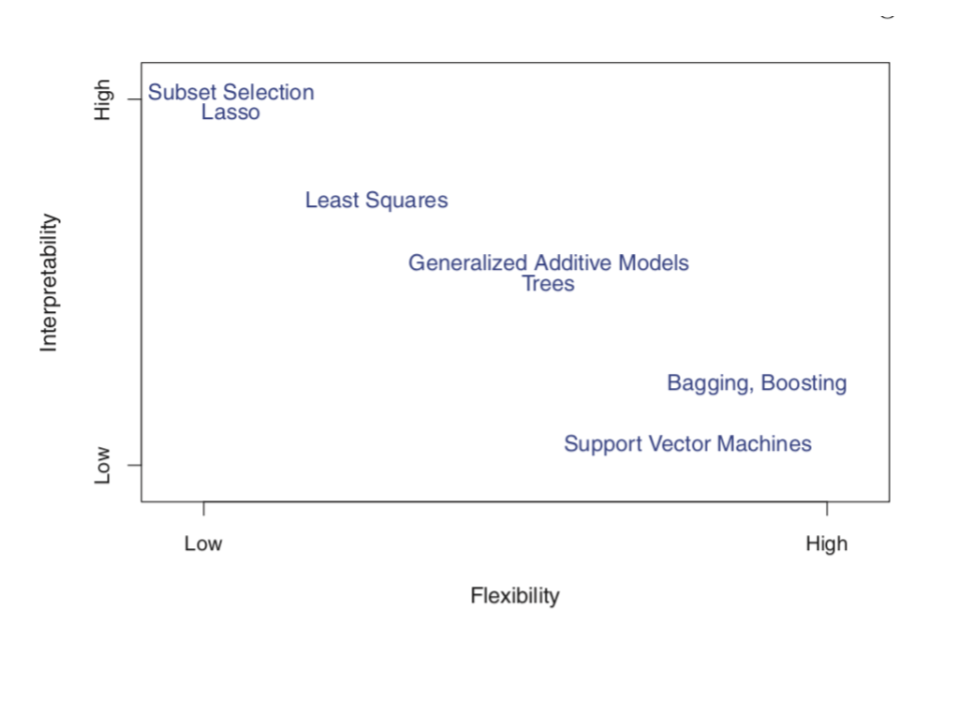
4. **Interpretability & flexibility**
When picking between different model building algorithms, there are several considerations, including *flexibility* and *interpretability*. Consider the following graphic from ISLR:
{width=100%}
a. Convince yourself that the placement of Subset Selection (e.g. backward stepwise), LASSO, Least Squares, and Splines (which is highly related to Generalized Additive Models) make sense. (We'll address other algorithms later this semester.)
b. Where would you place KNN on this graphic?
5. **Differences and similarities**
For each pair of algorithms below: try to identify a key *similarity*, a key *difference*, and any scenario in which they're "equivalent".
a. KNN vs LOESS
b. LOESS vs Splines
c. Splines vs least squares
d. least squares vs LASSO
6. **Pros & cons (there's a similar question on HW3)**
Summarize at least 1 pro and 1 con about each model building algorithm. You cannot use the same pro or con more than once!
a. least squares
b. LASSO
c. KNN
d. Splines
7. **Lingo (there's a similar question on HW3)**
In your own words, describe what each of these "everyday" words means in the context of ML algorithms:
- greedy
- biased
- parsimonious
- (computationally) expensive
- goldilocks problem
\
\
# Deeper Learning (OPTIONAL) {.unnumbered .smaller}
KNN, regression splines, and LOESS aren't the only flexible regression algorithms!
Chapter 7 of ISLR also discusses:
- piecewise polynomials (parametric)
- smoothing splines (nonparametric)
- generative additive models (nonparametric)
Read Chapter 7 of the book, and watch Prof Johnson's video on these topics to learn more:
[https://youtu.be/sYC3PuONUy8](https://youtu.be/sYC3PuONUy8)
\
Chapter 7.7 specifically provides more information about generalized additive models (GAM). These models take the ideas of splines and loess and combine them into one framework and allow each predictor to have a non-linear relationship. They are implemented in `tidymodels` but can be computationally intensive. They allow the relationships to either be estimated with loess or smoothing splines, both of which are non-parameter approaches.
In general, we can think of GAM as
$$y = \beta_0 + f_1(x_1) + \cdots + f_{p}(x_{p}) + \epsilon$$
where the functions $f_j(x)$ are estimated nonparametrically.
Chapter 7.5 provides more information about smoothing splines. In general, these techniques estimate the $f(x)$ by *penalizing* wiggly behavior where wiggliness is measured by the second derivative of $f(x)$, i.e. the degree to which the slope changes. Specifically, $f(x)$ is estimated to minimize:
$$\sum_{i=1}^n (y_i - f(x_i))^2 + \lambda \int f''(t)^2 dt$$
That is, we want $f(x)$ to produce small squared residuals ($\sum_{i=1}^n (y_i - f(x_i))^2$) and small total change in slope over the range of x ($\int f''(t)^2 dt$).
# Done!
- Render your notes.
- Check the solutions in the course website (Solution drop downs).
- If you finish all that during class, start your homework!