---
title: "Variable Selection - Part 2 (Notes)"
subtitle: "Stat 253"
author: "Your Name"
format:
html:
toc: true
toc-depth: 2
embed-resources: true
---
```{r part2-setup}
#| include: false
knitr::opts_chunk$set(
collapse = TRUE,
warning = FALSE,
message = FALSE,
error = TRUE,
fig.height = 2.75,
fig.width = 4.25,
fig.env='figure',
fig.pos = 'h',
fig.align = 'center')
```
# Notes & Discussion: Variable Selection {-}
Open the **Part 2** QMD to take notes.
Let's consider three existing variable selection algorithms.
Heads up: these algorithms are important to building intuition for the questions and challenges in model selection, BUT have major drawbacks.
\
## Algorithm 1: Best Subset Selection {.unnumbered .smaller}
::: incremental
- Build *all* $2^p$ possible models that use any combination of the available predictors $(x_1, x_2,..., x_p)$.
- Identify the best model with respect to some chosen metric (eg: CV MAE) and context.
:::
_Suppose we used this algorithm for our `height` model with 12 possible predictors: what's the main drawback?_
\
## Algorithm 2: Backward Stepwise Selection {.unnumbered .smaller}
::: incremental
- Build a model with *all* $p$ possible predictors, $(x_1, x_2,..., x_p)$.
- Repeat the following until only 1 predictor remains in the model:
- Remove the 1 predictor with the biggest p-value.
- Build a model with the remaining predictors.
- You now have $p$ competing models: one with all $p$ predictors, one with $p-1$ predictors, ..., and one with 1 predictor. Identify the "best" model with respect to some metric (eg: CV MAE) and context.
:::
__________________________________
_Let's try out the first few steps!_
```{r}
# Load packages and data
library(tidyverse)
library(tidymodels)
humans <- read.csv("https://mac-stat.github.io/data/bodyfat1.csv")
```
```{r}
#| eval: true
# STEP 1: model specifications
lm_spec <- linear_reg() %>%
set_mode("regression") %>%
set_engine("lm")
```
```{r}
#| eval: false
# STEP 2: model estimate (using all 12 predictors to start)
# Pick apart this code and make it easier to identify the least "significant" predictor!!!
lm_spec %>%
fit(height ~ age + weight + neck + chest + abdomen + hip + thigh + knee + ankle + biceps + forearm + wrist,
data = humans) %>%
tidy() %>%
filter(term != "(Intercept)") %>%
mutate(p.value = round(p.value, 4))
```
```{r}
#| eval: false
# 11 predictors (tweak the code)
lm_spec %>%
fit(height ~ age + weight + neck + chest + abdomen + hip + thigh + knee + ankle + biceps + forearm + wrist,
data = humans) %>%
tidy() %>%
filter(term != "(Intercept)") %>%
mutate(p.value = round(p.value, 4))
```
```{r}
#| eval: false
# 10 predictors (tweak the code)
lm_spec %>%
fit(height ~ age + weight + neck + chest + abdomen + hip + thigh + knee + ankle + biceps + forearm + wrist,
data = humans) %>%
tidy() %>%
filter(term != "(Intercept)") %>%
mutate(p.value = round(p.value, 4))
```
__________________________________
Below is the complete model sequence along with 10-fold CV MAE for each model (using `set.seed(253)`).
pred CV MAE predictor list
----- -------- ----------------------------------------------------------------------
12 5.728 weight, hip, forearm, thigh, chest, abdomen, age, ankle, wrist, knee, neck, biceps
11 5.523 weight, hip, forearm, thigh, chest, abdomen, age, ankle, wrist, knee, neck
10 5.413 weight, hip, forearm, thigh, chest, abdomen, age, ankle, wrist, knee
9 5.368 weight, hip, forearm, thigh, chest, abdomen, age, ankle, wrist
8 5.047 weight, hip, forearm, thigh, chest, abdomen, age, ankle
7 5.013 weight, hip, forearm, thigh, chest, abdomen, age
6 4.684 weight, hip, forearm, thigh, chest, abdomen
5 4.460 weight, hip, forearm, thigh, chest
4 4.386 weight, hip, forearm, thigh
3 4.091 weight, hip, forearm
2 3.733 weight, hip
1 3.658 weight
\
_DISCUSS:_
a. (Review) Interpret the CV MAE for the model of `height` by `weight` alone.
b. Is this algorithm more or less **computationally expensive** than the best subset algorithm?
c. The predictors `neck` and `wrist`, in that order, are the most strongly correlated with `height`. Where do these appear in the backward sequence and what does this mean?
```{r}
#| eval: true
cor(humans)[,'height'] %>%
sort()
```
d. We deleted predictors one at a time. Why is this better than deleting a collection of multiple predictors at the same time (eg: kicking out all predictors with p-value > 0.1)?
__________________________________
We have to pick just **1** of the 12 models as our final model.
That is, we have to pick a value for our **tuning parameter**, the number of predictors.
It helps to plot the CV MAE for each model in the sequence.
Here's what we saw above:
```{r}
#| eval: true
#| code-fold: true
data.frame(
predictors = c(12:1),
mae = c(5.728, 5.523, 5.413, 5.368, 5.047, 5.013, 4.684, 4.460, 4.386, 4.091, 3.733, 3.658)) %>%
ggplot(aes(x = predictors, y = mae)) +
geom_point() +
geom_line() +
scale_x_continuous(breaks = c(1:12))
```
_DISCUSS:_
a. Which model do you pick?!?
b. In the odd ["Goldilocks" fairy tale](https://www.youtube.com/watch?v=qOJ_A5tgBKM), a kid comes upon a bear den -- the first bear's bed is too hard, the second bear's is too soft, and the third bear's is just right. The second plot, below, illustrates a **goldilocks problem** in tuning the number of predictors in our backward stepwise model. Explain.
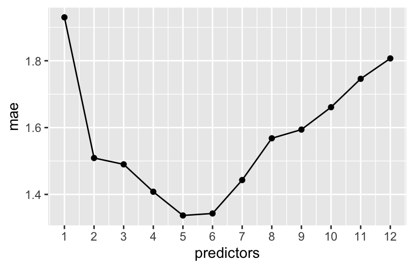
- When the number of predictors is too *small*, the MAE increases because the model is too....
- When the number of predictors is too *large*, the MAE increases because the model is too....
\
## Algorithm 3: Forward Stepwise Selection {.unnumbered .smaller}
_DISCUSS:_
- How do you think this works?
- Is it more or less computationally expensive than backward stepwise?
\
## Machine Learning vs Human Learning {.unnumbered .smaller}
When *tuning* or finalizing a model building algorithm, we (humans!) have our own choices to make.
For one, we need to decide what we prefer:
- a model with the lowest prediction errors; or
- a more **parsimonious** model: one with slightly *higher prediction errors* but *fewer predictors*
In deciding, here are some human considerations:
- **goal:** How will the model be used? Should it be easy for humans to interpret and apply?
- **cost:** How many resources (time, money, computer memory, etc) do the model and data needed require?
- **impact:** What are the consequences of a bad prediction?
\
_For each scenario below, which model would you pick: (1) the model with the lowest prediction errors; or (2) a parsimonious model with slightly worse predictions?_
a. Google asks us to re-build their search algorithm.
b. A small non-profit hires us to help them build a predictive model of the donation dollars they'll receive throughout the year.
\
## WARNING {.unnumbered .smaller}
Variable selection algorithms are a nice, intuitive place to start our discussion of model selection techniques.
**BUT we will not use them.**
They are frowned upon in the broader ML community, so much so that **tidymodels** doesn't even implement them!
Why?
- Best subset selection is **computationally expensive**.
- Backward stepwise selection:
- is **greedy** -- it makes *locally* optimal decisions, thus often misses the *globally* optimal model
- overestimates the significance of remaining predictors, thus shouldn't be used for inference
- Forward stepwise selection:
- is computationally expensive
- can produce odd combinations of predictors (eg: a new predictor may render previously included predictors non-significant).
# Exercises: Part 2 {-}
## Instructions {-}
- Goal: become familiar with new code structures (recipes and workflows)
- Ask me questions as I move around the room.
## Questions {.unnumbered .smaller}
The video for today introduced the concepts of **recipes** and **workflows** in the **tidymodels** framework. These concepts will become important to our new modeling algorithms. Though they aren't *necessary* to linear regression models, let's explore them in this familiar setting.
Run through the following discussion and code one step at a time. Take note of the general process, concepts, and questions you have.
**STEP 1: model specification**
This specifies the *structure* or general modeling algorithm we plan to use.
It does *not* specify anything about the variables of interest or our data.
```{r}
#| eval: false
lm_spec <- linear_reg() %>%
set_mode("regression") %>%
set_engine("lm")
# Check it out
lm_spec
```
**STEP 2: recipe specification**
Just as a cooking recipe specifies the *ingredients* and *how to prepare them*, a tidymodels recipe specifies:
- the *variables* in our relationship of interest (the ingredients)
- how to *pre-process* or wrangle these variables (how to prepare the ingredients)
- the *data* we'll use to explore these variables (where to find the ingredients)
It does *not* specify anything about the model structure we'll use to explore this relationship.
```{r}
#| eval: false
# A simple recipe with NO pre-processing
data_recipe <- recipe(height ~ wrist + ankle, data = humans)
# Check it out
data_recipe
```
**STEP 3: workflow creation (model + recipe)**
This specifies the general *workflow* of our modeling process, including our *model structure* and our *variable recipe*.
```{r}
#| eval: false
model_workflow <- workflow() %>%
add_recipe(data_recipe) %>%
add_model(lm_spec)
# Check it out
model_workflow
```
**STEP 4: Model estimation**
This step *estimates* or *fits* our model of interest using our entire sample data.
The model (`lm_spec`) and variable details (here just `height ~ wrist + ankle`) are specified in the workflow, so we do not need to give that information again!
```{r}
#| eval: false
my_model <- model_workflow %>%
fit(data = humans)
```
**STEPS 5: Model evaluation**
To get in-sample metrics, use `my_model` like normal.
```{r}
#| eval: false
# example: calculate of in-sample metrics
my_model %>%
glance()
```
To get CV metrics, pass the workflow to `fit_resamples` along with information about how to randomly create folds.
```{r}
#| eval: false
set.seed(253)
my_model_cv <- model_workflow %>%
fit_resamples(resamples = vfold_cv(humans, v = 10),
metrics = metric_set(rsq))
```
Then, proceed as usual... (`my_model_cv %>% collect_metrics()`, etc. )
# Done!
- Render your notes.
- Check the solutions in the course website (Solution drop downs).
- If you finish all that during class, start your homework!